Ziegler-Nichols Tuning Rules for PID
|
|
|
|
|
|
|
Introduction

(View more Control information)
A recent opinion piece published in the trade magazine Control Engineering proposed that the Ziegler-Nichols tuning rule would serve as the basis for a coming new generation of PID technology: "Improved performance, ease of use, low cost, and training will put Ziegler and Nichols in the driver's seat..." [1] Well, maybe so, but it seems to us that Ziegler-Nichols tuning is a very limited technology that is unlikely to be successful in that role. The rest of this article will explain why, exploring how to use the rule and where things can go wrong.
|
Related Product |
|---|
The time-honored Ziegler-Nichols tuning rule [2,3] ("Z-N rule"), as introduced in the 1940s, had a large impact in making PID feedback controls acceptable to control engineers. PID was known, but applied only reluctantly because of stability concerns. With the Ziegler-Nichols rule, engineers finally had a practical and systematic way of tuning PID loops for improved performance. Never mind that the rule was based on science fiction. After taking just a few basic measurements of actual system response, the tuning rule confidently recommends the PID gains to use. If results are what really matter, the results are... well, let's not talk about performance just yet.
Tuning rules simplify or perhaps over-simplify the PID loop tuning problem to the point that it can be solved with slide-rule technology. (Anybody remember the slide-rule?) Maybe that's not the best we can do today, but a weak alternative that is available can look a lot better than a good alternative that is not. That is why the Ziegler-Nichols Rule is still going strong today.
What is the Ziegler-Nichols Rule?
The Ziegler-Nichols rule is a heuristic PID tuning rule that attempts to produce good values for the three PID gain parameters:
- Kp - the controller path gain
- Ti - the controller's integrator time constant
- Td - the controller's derivative time constant
given two measured feedback loop parameters derived from measurements:
- the period Tu of the oscillation frequency at the stability limit
- the gain margin Ku for loop stability
with the goal of achieving good regulation (disturbance rejection).
When Does the Ziegler-Nichols Rule Work?
Tuning rules work quite well when you have an analog controller, a system that is linear, monotonic, and sluggish, and a response that is dominated by a single-pole exponential "lag" or something that acts a lot like one.
Actual plants are unlikely to have a perfect first-order lag characteristic, but this approximation is reasonable to describe the frequency response rolloff in a majority of cases. Higher-order poles will introduce an extra phase shift, however. Even if they don't affect the shape of the gain rolloff much, the phase shift matters a lot to loop stability. You can't depend upon a single "lag" pole to match both the amplitude rolloff and the phase shift accurately.
So the Ziegler-Nichols model presumes an additional fictional phase adjustment that does not distort the assumed magnitude rolloff. At the stability margin, there is a 180 degree phase shift around the feedback loop (Nyquist's stability criterion). A first order lag can contribute no more than 90 degrees of that phase shift. The rest of the observed phase shift must be covered by the artificial phase adjustment. The phase adjustment is presumed to be a straight line between zero and the critical frequency where 180 degrees of phase shift occurs. A "straight line" phase shift corresponds to a pure time delay. Is this consistent with the actual phase shifts? Well, probably not, so hope for the best.
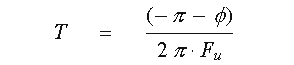
To summarize, then, the Ziegler-Nichols rule assumes that the system has a transfer function of the following form:
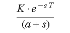
The model matches the system response at frequencies 0 and at the stability limit, and everything else is more or less made up in between. If the actual system is linear, monotonic, and sluggish, it doesn't make much difference that the model is fake, and results are good enough. If the actual system does not match the assumed model adequately, then sorry, you're on your own.
How Do You Measure the Response Parameters?
You don't need to determine all of the model parameters to apply Z-N tuning, but if you wanted to do so, here is how you could measure them.
Perform a frequency response test on the system, to determine the gain magnitude and the phase shift as a function of frequency. You can take your system offline, attach a signal source, and attach a data acquisition system to measure input and output data sets. Or, if you are smarter about it, you can measure your system response online [5] while the PID loop is operating.
Given the magnitude and phase open-loop response curves of the plant, you can fit the assumed model in the following manner.
-
The ratio of output level to input level at low frequencies determines the gain parameter
Kof the model. -
Observe the frequency
Fuat which the phase passes through -pi radians (-180 degrees). The inverse of this frequency is the period of the oscillation,Tu. -
Observe the plant gain
Kcthat occurs at the critical oscillation frequencyFu. The inverse of this is the gain marginKu. -
Apply the frequency
Futo the plant first order lag terms to solve for the model'saterm.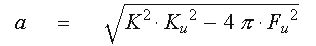
-
Evaluate the phase shift of the lag stage by substituting
Fuinto the first-order lag model.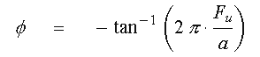
The rest of the 180 degrees of phase shift are assigned to the pure time delay term.
In practice, you don't need to construct the complete model, and you can stop after completing step 3 above.
Applying the Tuning Rule
Use the values of Ku and Tu to determine values of PID gain setting according to the following tuning rule table. [4]
| Rule Name | Tuning Parameters |
|---|---|
| Classic Ziegler-Nichols | Kp = 0.6 Ku Ti = 0.5 Tu Td = 0.125 Tu |
| Pessen Integral Rule | Kp = 0.7 Ku Ti = 0.4 Tu Td = 0.15 Tu |
| Some Overshoot | Kp = 0.33 Ku Ti = 0.5 Tu Td = 0.33 Tu |
| No Overshoot | Kp = 0.2 Ku Ti = 0.5 Tu Td = 0.33 Tu |
Why are there multiple rules? Well, remember, all of these are just heuristics. Some people find the transient overshoot levels of the classic Z-N rule excessive and will accept a slightly longer transient interval in exchange for smoother settling. Some people find that the Z-N classic rule doesn't quite achieve the disturbance rejection goals that were the original objective. Pick the rule that you think works best for you. This might be an ad-hoc solution, but it is an ad-hoc solution that can be applied systematically.
A Tuning Example
The following illustration shows plotted data of the
system's open loop frequency response, gain and phase, as
captured by an automated online test performed by the PIDZMON command, [5] described in another
note on this site. The green lines and the magenta line have
been superimposed on the screen capture image.
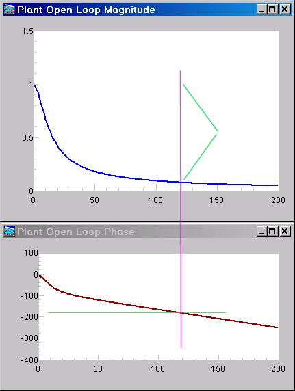
Tracing along the horizontal green line in the lower plot, we can see that the critical 180 degree phase shift occurs at a location that is about 120/200 of the Nyquist frequency. Given that the sampling rate was 50 Hz, this would correspond to a critical frequency 0.6 * 1/2 * 50 Hz, or 15 Hz. The corresponding critical time interval is the inverse, Tu=0.06666 seconds.
Tracing vertically at this frequency along the magenta line, the upper plot shows that the open loop gain of the plant has rolled off to a value of about 0.09 here. Applying a controller gain of about 11.1 as indicated by the green brackets would result in a net loop gain 1.0 with a phase shift of 180 degrees, so the system would be operating with sustained oscillation at the stability limit. Thus, the gain margin Ku is about 11.1.
Choosing the classical Ziegler-Nichols tuning rule, we would then determine that the PID gains should be
  loop gain Kp = 0.6 * Ku = 6.7
  integral time constant Ti = 0.5 * Tu = 0.033
  derivative time constant Td = 0.125 * Tu = .0083
Why Do We Keep Hinting That Results are Lousy?
Among the reasons:
- Garbage-in, garbage out. If you believe (or hope) that the tuning rule assumptions are good, but they are not, anything could happen.
- Limited applicability. Even if you are not fooled when the assumptions do not apply, there might not be much you can do about it.
- Inconsistent design goals. The Ziegler-Nichols tuning rule is meant to give your PID loops best disturbance rejection performance. This setting typically does not give very good command tracking performance. It is easy to pick a tuning rule that is poor for the application, and you might not realize it.
- Overly aggressive gains. Tunings based on a continuous system analysis can produce erratic behaviors with a discrete controller. When the pure delay parameter is small, the critical frequency can be too close to the Nyquist limit, in a range where a zero-order hold results in choppy signals.
- Dependence on non-reality. The ability of the model to predict good tunings is highly dependent on the unrealistic pure time delay assumption, which can perform rather badly, for example, when phase shift results from a complex pole pair.
These problems and others have prompted other tuning strategies. There is no arguing with success, but success is not guaranteed, so you have to be careful.
Conclusions
Tuning rules such as the Z-N rule and its variants are embedded into well established, very convenient generalized controller products. All have the same advantages and disadvantages: If the rule works, great! Use it. If it doesn't work... then what are you going to do?
Unfortunately, we cannot recommend the Z-N rule or related tuning rules strongly. The idea is straightforward but the application is tricky. Ordinarily, you need to test your system offline and instrument it for special response tests. DAP-based controls can perform the tests online and deliver the response curves [5], maintaining control and never missing a tick. While this adds no new fundamental capabilities, at least it represents a shift from a manual offline measurement process to an automated online one. This seems to be what the Control Engineering article praises as the ultimate in technology. While we can consider the Ziegler-Nichols rule helpful, there are more robust alternatives available today. You can test the method using your DAP system. Download the free command code and find out for yourself.
Footnotes and References:
- "Getting in tune with Ziegler-Nichols," Thomas R. Kurfess, PhD, in the Academic Viewpoint column, Control Engineering magazine, Feb 2007 issue, p. 28, http://www.controleng.com/.
- The classic original paper: "Optimum settings for automatic controllers," J. B. Ziegler and N. B. Nichols, ASME Transactions, v64 (1942), pp. 759-768.
- A more recent survey that covers the Ziegler-Nichols and Kappa-Tau tuning rules: "Automatic Tuning of PID Controllers," Karl J. Åström & Tore Hägglund, Chapter 52, The Control Handbook, IEEE/CRC Press, 1995, William S. Levine ed.
- Selected from the tuning rules listed in the paper "Rule-Based Autotuning Based on Frequency Domain Identification," Anthony S. McCormack and Keith R. Godfrey, IEEE Transactions on Control Systems Technology, vol 6 no 1, January 1998.
- For more information about obtaining frequency response curves automatically, see the article A Self-Testing PID Loop on this site.
Return to the Control page.