A Self-Testing PID Loop

Introduction

(View more Control information or download the preliminary implementation.)

This note offers a new kind of solution for the ongoing problem of online monitoring and tuning of PID loops.

There are reasons why some of the control techniques discussed in other pages on this site are not always appropriate. Sometimes, PID controls are a devil known while other techniques are a devil unknown. That is, whatever the appeal of finding something better, the costs of changing and being wrong are too high. In many other cases, PID controls have already proven themselves to be perfectly adequate, and, given that they are perfectly adequate, nothing more complicated is justified.

For whichever reason, when PID controls are the strategy of choice, it is still true that conditions can change. Staying "well tuned" is very important. Poorly tuned loops can have a significant economic impact.

A Disturbance in the Force

One of the most basic strategies for evaluating loop tuning involves measuring loop gain and phase shift as a function of frequency. Unfortunately, it is not possible to measure frequency response if frequencies are not present to measure. If natural disturbances are not present, artificial disturbances must be introduced.

Considerations when performing a loop response test:

How can you connect and disconnect the test instruments for generating appropriate stimulus?
How are tests conducted?
How are test results recorded and logged?
Do you have to take the system offline? Can it run offline?
How is the gain/phase analysis performed?
The controller gain settings must be adjusted, and then...
Performance of the new tuning must be verified.

While the PID control itself might be simple, the amount of effort to support response testing can be very high. The goal of the self-testing PID control is to make this much easier, by integrating important parts of the testing and data pre-processing into the controller itself. For a DAP-based control:

The Data Acquisition Processor (DAP) board itself is the measurement instrument. It is always there and always ready.
To run a test at any time, just send a message.
Communication channels transfer messages and return the measurement data sets.
Tests can be run without taking the system offline.
The results are fully processed, in the form of gain/phase curves that can be displayed or logged.
Loop gain settings are installed by sending command messages, using the same supervisory communication channels.
The process is fast and automatic. You can repeat any desired number of times to adjust and verify.

Excitation Signals for Test

To measure frequency response, it is necessary to compare the output at a given frequency to the excitation input at that same frequency. Conventional practice does a generally bad job of exciting all of the frequencies in the relevant band. To explain this statement, it is first necessary to consider what "the relevant band" is, with respect to a PID control loop. Nyquist's criterion says that a signal cannot be reconstructed unless there are at least two samples per cycle for the highest frequency present in the signal band. But most digital implementations of PID controllers do not use the elaborate interpolation filters necessary to reconstruct a signal from sparse sample sequences. What is done in practice?

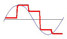
The output values are sent to a first-order hold, resulting in a stair-stepped output sequence. This illustration shows the update sequence for a frequency that, according to the theoretical limits, is more than a factor of 2 lower than necessary. Does the stepped waveform look anything like the desired continuous waveform?

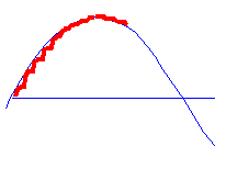
Using a simple first-order hold, it is highly desirable to have 10 or more samples along each quadrant of the waveform.

10 or more samples per quarter wave means 40 or more samples per complete wave cycle, or a factor of 20X oversampling, or 5% of the theoretical limit. Frequencies above 10% of the Nyquist limit can be trouble.

We also do not want abrupt jerking responses from the system. We expect the controlled plant to have a lowpass characteristic so that any small step-edges are smoothed out. (For one thing, if the plant does not have a lowpass characteristic, the ordinary tuning rules do not apply.) This means that frequencies much more than 10% of the Nyquist limit also are not desirable in the system output signals. If the loop response exhibits high levels of signal energy in at higher frequencies, the sampling rate is probably too low.

Given this information, consider the "industry standard" with regard to PID loop tests. In describing the advanced version of their loop-test software, the ExperTune Web site [1] shows the following list of choices for tuning excitation signals.

Open loop step

Closed loop step (controller in automatic)

Open loop pulse

Closed loop pulse (controller in automatic)

Pseudo random data

Open loop doublet pulse

This is a quite good coverage of the test signals actually employed in practice. Let's assess the relative strengths and weaknesses.

Step response tests have some serious drawbacks. A step edge introduces broadband excitation, but the edge that excites high frequencies is very short duration. A short time duration means poor frequency resolution. A step test results in a long term level disturbance in the process, which can be a problem when testing online.

Pulse response tests first apply and then remove a large command displacement. Because the disturbance is not sustained for very long, the magnitude of the disturbance can be larger, reducing the long-term displacement of the operating state. In higher frequency bands, there is a rough doubling of the excitation energy because of two transitions rather than just one. However, the short-term excitation must be large to see much response at lower frequencies. A large disturbance can sometimes have unacceptable side effects.

Doublet response tests, in effect, are pulse tests split into two parts, a hard knock in one direction, followed by a hard knock in the other. The offsetting knocks will not upset the process level as much, so they can be larger, while providing more broadband disturbance energy. This is an improvement for online testing because of less net displacement in the operating state of the running process, but it has the same problem of high-energy disturbance like the other impulse test methods.

Random excitation tests provide an alternative that excites the system response over a wide band. White noise distributes energy equally at all frequencies — at least in the limit it does. As we have just seen, this means that the great majority of the disturbance energy is in the wrong bands and not helpful. But worse, the results of random noise tests are — well, very random. While the band coverage is pretty good, the variances in the results can be quite awful.

Magnitude/Phase Response

Rather than exciting everything, the Microstar Laboratories self-testing PID controller provides a built-in disturbance signal generator that excites only the frequencies that you need, in a manner almost free of random noise. Because it is non-random, and has an exactly known energy at every frequency, it produces repeatable results.

Excitation frequency band
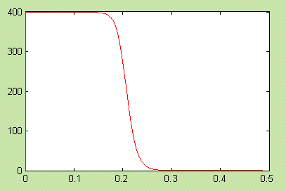
Excitation frequency response

The test signal has some highly desirable properties:

The signal energy is limited to below 20% of the Nyquist frequency. (Of course, that is wider than the desirable operating band! For testing, the extended band helps for characterizing the plant rolloff.)
There are no impulses, which could result in hard shocks to the system and undesirable high-band noise.
The disturbance signal is completely balanced, so it can ride on top of an existing steady-state command signal in closed loop operation – the loop does not need to be taken offline.
Excitation energy is evenly distributed through the relevant band.
Disturbance energy is distributed over time, so the magnitude can be much lower than in impulse tests, allowing a larger net energy with a smaller net process disruption.
The phases of the frequencies in the relevant band are selected to minimize peaks, for best signal to noise ratio in the limited converter range.

Because the injection signal is predetermined, computing the magnitude/phase response is extremely simple. The system is operated at a steady command level. A signal is injected at an appropriate location in the loop, added to the signal already present in that path. A block of response data is collected, and an FFT analysis is applied. The system is in quasi-steady state, hence frequencies other than zero are the result of the test excitation, plus whatever small amounts of noise are present. For the relevant frequency band, the ratio of response amplitude to (constant) excitation amplitude determines gain. The difference between the output phase angle and the (predetermined) excitation phase angle determines phase response.

It might first appear that injecting a disturbance signal into the plant control input and monitoring the plant output would yield the open loop response of the plant, riding on top of a constant level. This is not true, however, because it does not take into account signal propagation around the closed loop. Consider the following diagram with PID controller C and plant P.

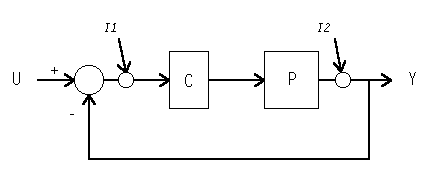
Tracing the signals around the loop, we will find that the two transfer functions of interest are:

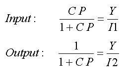
Input injection: the command transfer function: For accurate tracking of the input command signal I1, the response Y should sustain over a moderately wide band without excessive phase distortion.
Output injection: the disturbance rejection transfer function: A disturbance signal I2 injected into the output Y should be cancelled by the feedback action as quickly as possible to restore operation at the setpoint level. The lower the response curve, the better.

Skipping a lot of mathematical details, we can derive from the two injection experiments the command transfer function, the output rejection function, and the plant open loop transfer function. The latter characteristic is of special interest, because it indicates the critical frequency for stability in closed loop operation. These response curves are the delivered results.

"Okay, I have transfer characteristics. Now what?"

Unfortunately, the rest of the story is not pretty. Nyquist's stability criterion says that the system is at the margin of stability if the loop gain is 1.0 at a phase shift of 180 degrees. That's all very fine, but you don't want to operate at the ragged edge of instability. First, you must reduce the gain to provide a suitable stability margin. Then, you can apply integral correction to reduce tracking errors and improve rejection response, and derivative correction to improve the phase margin. Qualitatively, this all makes sense. But quantitatively...

That's where the tuning rules come in. If you employ the usual fixed rules, they are based on assumptions that the system is well approximated by a first-order lag (to approximate the lowpass roll-off characteristic) and a pure time lag (to approximate phase shifts due to higher-order effects). If these assumptions don't apply, the rules won't help you much. So assume that the rules work well enough. The tuning rule that you apply will prescribe how to set the PID gains as a compromise between stability, responsiveness and noise rejection.

For example, determine from the plant phase curve the frequency at which the phase shift is 180 degrees. The inverse of that critical frequency is defined as critical time Tu. Determine the plant magnitude gain at the critical frequency. The inverse of this gain is defined as Ku, the critical loop gain. Given these two parameters, the classic Ziegler-Nichols tuning rule for good disturbance rejection at the expense of some overshoot in response to setpoint change is:

  K  =  0.6*Ku
  Ti =  0.5*Tu
  Td =  0.125*Tu

This rule was devised with continuous controllers in mind. In discrete controllers, it tends to excite high frequencies too much. It also tends to produce a nasty overshoot in response to setpoint changes. The "some overshoot rule" will track changes to the setpoint somewhat better, while not rejecting disturbances as well:

  K  =  0.33*Ku
  Ti =  0.5*Tu
  Td =  0.33*Tu

See the paper cited below [2] for a survey of candidate tuning rules. Do these rules work well? No, not really. But what else are you going to do? That, it seems, must be a topic for another day. If you know from experience how to use the curves to find good gain setting for your particular system, apply your experience. You might also find that the zero-shaping parameter of the PIDZ command (see the related article [3] on this site) helps to moderate transient response while keeping loop gains high.

Implementation

The self-testing features have been integrated with the PIDZ command to produce the PIDZMON command. PIDZMON retains all of the PID-related features of PIDZ.

The self-testing process requires three additional command parameters for configuration.

request pipe: Provide a pipe to transfer requests to initiate an injection test cycle. Place an arbitrary number into this pipe, for example using a FILL command. The PIDZMON command will remove this value and begin the injection test. Only one test can be active on a loop at any one time, so until the test is completed, any additional requests are removed and ignored.
excitation scaling: Select the magnitude of the disturbance that your system can tolerate. You want it as large as possible to get good resolution and accuracy; but you want it as small as possible to avoid disruption to the online process. In addition, for PID settings with high gains, you will want to avoid saturating the controller command signal. You will have to find the appropriate compromise. For example, suppose your system operates at about level 16000 (half of the converter's maximum positive range), and that it can withstand disturbances of about +-1000. Compared to the converter's +-32000 range, this is roughly 3%, so specify a 0.03 excitation scaling level.
response characteristic pipe: Provide a pipe to receive the transfer characteristic data. The characteristics are provided as five data blocks, each consisting of 200 FLOAT values. The first two blocks are the command response transfer magnitude and phase. The second two blocks are the plant open loop transfer magnitude and phase. The last block is the output injection magnitude. Angles are reported in degrees.

You might have wondered: with all of the DSP analysis and data transport activity going on, wouldn't that extra computation interfere with updates of the PID loop, making the controller response erratic, possibly even resulting in loss of loop control? If this didn't trouble you, it should have. It is not a problem, however. Blazing speed is what DAPs are all about. The FFT computations are completed in a fraction of a millisecond. That means, as long as the update intervals are one millisecond or longer, control updates are never missed, and never late, not even during the most intense parts of the data analysis. Your system will never lose synchronization, and never lose data.

Disclaimers

The PIDZMON command is currently under consideration as a commercially supported product. The version provided to accompany this note is experimental. It is not fully developed, and not, a supported Microstar Laboratories product. If errors of about 2% would be critical to your tuning decisions, you should not use this command. Systems with characteristics that do not comply with the usual PID tuning rule assumptions of a linear, lowpass plant characteristic with time delay and well damped first or second order rolloff might not be characterized accurately.

With the above understanding, it might still be true that the results are better than anything previously available. If you would like to obtain a copy for test and evaluation, go to the download page on this site.

Because this module does not yet have the thorough testing and field application experience of supported DAPL system commands, before you consider using this command in your own field applications, you must be willing to do your own thorough testing and accept the risks involved.

Observations and Conclusions

The payoff for using Data Acquisition Processor (DAP) boards in control applications comes when you can take advantage of the extensive additional capabilities that the DAP has to offer. DAP boards were originally intended for data capture and real-time data analysis, with control applications secondary. This can also go the other way. DAP boards can also be used effectively for reliable and flexible control applications, with the data capture and real-time analysis as secondary features.

The DAP itself is a measurement instrument and a sophisticated signal generator. In effect, a control loop driven by a DAP is already fully instrumented and ready to test at any time, on request. The PIDZMON command includes a sophisticated, balanced, non-impulsive signal generator, but as they say, "It's all just software." It takes advantage of the largely unused capacity of the DAP processor for signal generation and data analysis. With a basic PID control device, you are fortunate to have accessible signal terminals for attaching test instruments — and the instrumentation is priced separately.

We have been referring to sampling rates on the order of 1000 updates per second, but there are many systems for which PLC update rates of 60 times per second are considered screaming fast. Whether processing is for one loop updated 1000 times per second or 16 loops updated 60 times per second makes no difference to the DAPL system.

Finally, we can note that independent DAP-based controllers for multiple loops would reside in an industrial PC host, such as the Microstar Laboratories DAPserver. The host can then act as a communication hub. Study of the response data, decisions about changing loop gains, data logging, and observation of process change over time – these can all be done from a remote location, without taking systems offline.

Footnotes and References:

See the state of the art in PID loop tuning, with dozens of useful articles, at the ExperTune web site. Is our DAP-based method better than other test methods? We think so, but remember, conventional PID control systems don't support it. Professional analysis packages such as the ExperTune software could do the analysis, but that would be pointless without the data.

Rule-Based Autotuning Based on Frequency Domain Identification, Anthony S. McCormack and Keith R. Godfrey, IEEE Transactions on Control Systems Technology, V. 6, No. 1, Jan 1998, pp. 43-61. They suggested the idea of the pre-designed excitation signal, but applied a coherence analysis instead of a direct transfer function analysis to the data sets. Their approach is entirely credible, and has some advantages for detecting problems from nonlinearity. Their paper also provide an excellent survey covering a number of heuristic tuning rules.

PIDZ - A PID Controller With Zero-Shaping on this site provides more information about PID transient response and tracking.

Return to the Control page. Or download the preliminary implementation.