Cold junction compensation

Home

Products

Applications

Thermocouple Cold Junctions

Temperature Measurement

Calibration Overview

Thermocouple Example

Thermocouple Calibration

The terms hot junction and cold junction, as applied to thermocouple devices, are mostly historical. You don't need to have any junctions to get thermocouple effects. If you heat one end of a metal conductor and hold the other end at a constant reference temperature, two important things occur.

Heat flow. There is a thermal gradient, so heat flows from the hot end to the cold end. With small-gage thermocouple wire, very little thermal energy actually reaches the cold end, and the thermal gradient is typically not constant along the wires because of heat loss.
Seebeck effect. Energetic electrons at the hot end diffuse toward the cold end, pushing less energetic electrons along with them, resulting in a higher static potential at the hot end relative to the cold end. The larger the temperature gradient, the larger the potential difference. (There are additional contributing effects when dissimilar materials are joined.)

In practice, it is difficult to measure the Seebeck effect directly. When you attach measurement probes, there is a thermal difference across the probe leads, producing additional thermocouple effects that interfere with the measurements.

Classical thermocouple loop configuration

To make the thermal effects measurable, two different metal conductors are used. They must be chemically, electrically, and physically compatible. They produce different electric potentials when subjected to the same thermal gradient.

In the classical configuration, the dissimilar thermocouple wires are welded together at the measurement end (hot junction), and again at the reference end (cold junction), forming a loop. The hot junction assures that the potential at that point matches in the two metals. Immersing the reference-end junction in an ice-water slurry assures that the temperature gradients are the same across both materials. The ice-water slurry establishes a reference temperature at 0 degrees C.

Illustration of closed loop
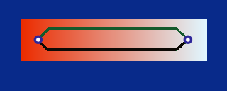
Figure 1 - dissimilar metals form loop, two junctions

Welding the thermocouple wires at the cold junction also equalizes the potentials there. To make the potential difference observable again, it is necessary to break the loop. Pick a location in one of the thermocouple wires where the temperature matches the temperature of the measurement leads. Break the loop there, and attach matching leads to the two sides of the gap to measure the potential.

Illustration of closed loop
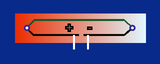
Figure 2 - potential difference where loop is broken

By maintaining uniform temperatures where the leads connect, thermal gradients are unaffected.
By avoiding thermal gradients across lead wires, stray thermocouple effects are kept small.
By matching the leads well, any residual effects cancel out of differential measurements.

Cold junction in practice

Maintaining an ice water slurry and actual cold junction is rarely feasible. Typically, the cold junction is omitted, and the potential is measured directly across the two terminal ends of the thermocouple wires at ambient temperature. For historical reasons, we speak of the terminal ends of the thermocouple wires as the cold junction, despite the fact that there is no longer an intentional junction. (For the same historical reasons, we refer to the measurement junction of the thermocouple as the hot junction even if it is used to measure below-zero temperatures.) The measured potential indicates the temperature difference between the hot junction point and the unknown cold junction terminals. To complete the temperature measurement, you must determine the terminal temperature in some manner.

Illustration of closed loop
Figure 3 - omitting the physical cold junction

Cold Junction Compensation

There are two commonly used approaches.

Simulate the potential effects that would result for a thermocouple wire pair between the terminals, at their measured temperature, and another junction at a reference temperature of 0 degrees. Measure the potential across the thermocouple wire pair in series with the simulated potential. Apply the linearizing curve to the sum, thus obtaining an estimated absolute temperature directly. This is known as cold junction compensation. Usually, the simulation is done electronically with specialized integrated circuit devices.

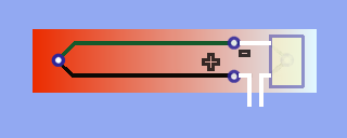
Figure 4 - electronic cold junction compensation

This approach makes two approximation errors, one for estimating the cold junction temperature, and one for approximating the effects on junction potential. Beyond what is already built into the electronic simulation, calibration is tricky and probably limited to offset adjustment.
Independently measure the temperature of the cold junction. Measure the thermocouple potential and apply conversion curves to determine the temperature difference across the thermocouple. Then add the known cold junction temperature to the measured temperature difference to determine the absolute temperature measurement.

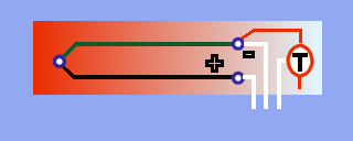
Figure 5 - independent cold junction measurement

This approach uses one less estimate, but it still depends on accurate measurements of the cold junction temperature.

LT1025A solid state temperature measurement devices are available on MSTB009 termination boards and optionally available on MSXB037 analog expansion boards for measuring the cold junction temperature when thermocouple wires connect directly to the terminals on the boards. Any errors in reading the cold junction temperature will appear directly as errors in the final temperature measurement. The readings are 10 millivolts per degree centigrade absolute temperature. Install a header plug on your board to activate temperature measurements that you can route directly into the THERMO command provided by the DAPL system.