Calibrating Thermocouple Sensors
|
|
|
|
|
|
|
Calibrate Thermocouples


The potential produced by a thermocouple as a function of temperature difference between its two ends is very nearly linear, over a very wide range. The following curve is the "standard response curve" for a type-K thermocouple.
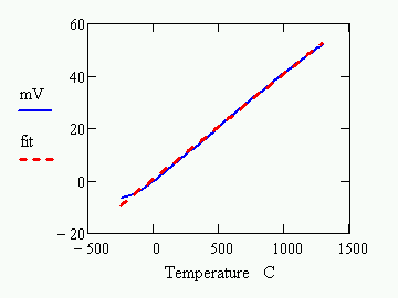
The deviations from perfect linearity are significant, however. If you compare the curve to a best fit line, you will find the following differences over the full temperature range.
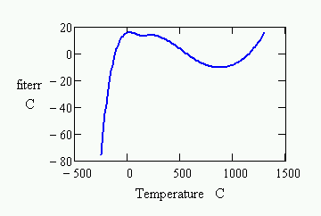
The differences are significant enough that most applications need a correction to obtain acceptable measurement accuracy. For moderate accuracy, you can assume that standard device curves match your actual thermocouple exactly, and use the standard response curves. This can yield a measurement accuracy within a few degrees. If you calibrate, you obtain maximum measurement accuracy for your individual thermocouple device, and also correct for any offset and gain errors present in your measurement system.
Linearization Functions for Thermocouples
The most common way to linearize the thermocouple response is to use a relatively high-order polynomial function. The function is dominated by the linear terms, but higher-order terms add the local curvature for a better fit. Standard linearizing curves are constructed in this way.
Individual thermocouples are very stable and repeatable, even if they do not match the standard curves exactly. Over a limited temperature range, it is possible to reduce the measurement error to about 1 degrees C using a well-calibrated lower-order polynomial curve.
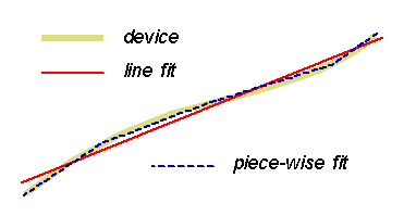
The nonlinearity in thermocouple characteristic curves
is almost unmeasurable over a bounded temperature
range. Piece-wise linear approximations are a good alternative
to the explicit function models. The DAPL system's THERMO command uses the piecewise curve strategy, matching the
standard curves within a fraction of a degree.
Calibrating a polynomial model
You will need to determine the order of polynomial to use. For a reduced temperature range (a few hundred degrees) a third or fourth order polynomial fit should provide sufficient conversion accuracy. For example, the following third-order polynomial matches the standard curves for a type-K thermocouple with error less than 0.1 degrees C through the range -45 degrees C to +150 degrees C.
T  =  -0.01897 + 25.41881 V - 0.42456 V2 + 0.04365 V3
where V is voltage in units of millivolts
and   T is temperature in degrees C
You can modify the coefficients slightly to make the conversion curve match an individual device's response for best accuracy. The calibration data must be captured very carefully, but the process is straightforward.
- Establish stable temperatures throughout the full operating range that you intend to cover.
- Measure each temperature carefully using an accurate measurement standard.
- Take many measurements of the noisy thermocouple potential at each temperature point, averaging these measurements to reduce noise.
- Collect the temperature-potential data pairs, and apply a least-squares curve fitting analysis to obtain a polynomial that best predicts the temperature given the junction potential.
Calibrating a piece-wise linear model
It typically takes about 20 linear pieces to adequately
approximate thermocouple standard curves. For better accuracy,
more pieces should be used. Assume that the number of sections
is increased to 40, then reduce the number of pieces in
proportion to the fraction of the total range your application
needs. So for example, a type-K thermocouple has a range of
about 1600 degrees C. A temperature range of 200 degrees C is
1/8 of that, so a calibrated model with about 40/8 = 5
pieces should produce good conversion accuracy.
Knowing that the response will be nearly linear for each of
the pieces, you don't need to measure everywhere as you do with
a polynomial fit. For an N-piece model, measure at the
two ends of the temperature range, and also at N-1
roughly evenly-spaced intermediate points. Use the same
precautions as with a polynomial fit, allowing temperatures to
stabilize, and taking multiple measurements at each selected
point for noise reduction. You can then code the
monotonically-increasing voltage terms as a vector of input
x-values, and the corresponding temperature levels as
a vector of y-values. Provide these two vectors to
the INTERP command to evaluate your piecewise
curve at any point.
Calibrating cold junction effects
You can read more about the principles and application of cold junction compensation in another page on this site.
There are some practical limitations on the accuracy you can achieve when using the LT1025A temperature measurement devices available on MSTB009 termination boards, and optionally available on MSXB037 analog expansion boards.
- The baseline temperature measurement error of the chip is 0.5 degrees C.
- Even when you bring the thermocouple wires all the way to termination board terminals, physically close to the location of the temperature measurement chip, it is difficult to maintain perfectly uniform temperatures across the termination board. You are doing very well if you can hold this error to an additional 0.5 degrees C.
- Calibrating the sensor chips would require controlling the board environment to a number of stable and accurately measured operating temperatures. This is probably infeasible.
The bottom line: any errors in reading the cold junction temperature will contribute directly to errors in the final temperature measurement. Expect at least 1 degree error from cold junction measurements when using the on-board temperature memeasurement circuits.
For better accuracy, you will need better control and calibration of your cold junction measurements. An application using a separate calibrated temperature sensor for best cold junction measurement accuracy is described in an application note on this site.
Thermocouple applications that do not calibrate cannot do much better than the THERMO command provided by the DAPL system. For evaluating customized piecewise-linear curves, you can use the INTERP command, also provided by the DAPL system. For evaluating polynomial models, you can use the generic polynomial evaluator command GENPOLY available on this site. Or for a special case that also covers cold junction compensation, you can use the THERMOPOLY command available on this site.