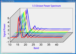
Versatile FFT Supports
Accurate 1/3 Octave Analysis
Technical Note TN-257 Version 1.0
For highly-precise 1/3 octave analysis of audio signals
Introduction
When Agilent chose to retire the classic HP 3582A audio spectrum analyzer, high-quality audio spectrum analysis suddenly became a lot harder. This article discusses a way to configure a general-purpose xDAP measurement system for this purpose — discovering higher levels of performance, lower cost, and new opportunities for measurement system automation.
Overview of Octave Analysis
Mathematically, a pair of sine waves at 80 and 80+10 cycles per second, or at 8000 and 8000+10 cycles per second, are equally distinguishable. As audio signals, however, the first pair would be perceived as significantly different tones to a listener, while the last pair would be virtually indistinguishable. Pitch is perceived as changing with the ratio of frequencies, not by linear increase in cycles per second. In an audio signal, tones one octave apart differ by a factor of 2 in frequency. As you go from lower to higher frequencies, each successive octave band doubles in width.
To more naturally group frequencies of audio signals, so that the distributed signal power scales better for analysis, measured signal power can be combined within each octave. This is known as octave analysis. For purposes of analyzing audibility rather than equipment performance, A-weight filtering [2] is often combined with the octave analysis, so that instead of showing the actual signal power, each octave shows approximately the perceived signal loudness in each octave.
The audible range is spanned by just a few octaves, so partitioning the spectrum octave-by-octave produces a relatively coarse distribution. Resolution is improved by breaking the octave bands into sub-octave bands, preserving the logarithmic band spacing. For the conventional case that octaves are separated into 3 parts, each successive 1/3 octave band increases in width by a factor of 1.25992. Though the relative widths are fixed mathematically, standards [3] define nominal locations for these bands — useful for labeling purposes.
Methods of Octave Analysis
The traditional way for instruments to perform an octave analysis was to pass the signal through a bank of analog bandpass filters, each filter responding to a narrow portion of the spectrum. The total signal power in each band is then proportional to the square of the signal magnitude in each band.
Designing these analog filters well — so that they precisely align to the desired band centers, roll off at precisely the right places, include all spectrum energy, avoid excessive overlap, and scale gains to correctly reflect the signal power in each band — turns out to be a remarkably difficult design problem. There is little wonder that high-quality spectrum analyzer instruments have always been relatively expensive.
Digital processing technology is a practical alternative today. Digital filtering can approximate the behaviors of the traditional analog filters. This approach also turns out to have its own share of difficulties, however. Analog filter banks have a natural logarithmic character, but digital filters do not. The easy methods for mapping the analog designs to digital designs do not produce good results at the band edges, and considerable effort is necessary to individually tune each filter characteristic. Another difficulty is the time/resolution tradeoff. The sampling rates necessary to capture high frequency information produces excessive data sets at low frequencies, so the design turns into a multi-rate as well as a multi-band problem.
The approach discussed in this note is based on FFT analysis. This shares the resolution and time scale difficulties of other digital approaches. However, it is appealing because the difficult filter design work is eliminated. An FFT acts like a huge bank of very precisely tuned digital filters. The challenge is to properly identify the desired 1/3 octave bands.
Preprocessing? or Postprocessing?
Performing the octave analysis on a DAP sometimes makes good sense; sometimes it does not. It depends on the application.
If the venerable HP analyzer instruments had produced only a stream of raw measurement numbers, not an immediate presentation of the spectrum results, it would have been considered a disastrous failure. Yet, that kind of thing is tolerated as the norm in the present day of "virtual instruments".
You can do some really advanced analysis using the appropriate GUI tools in your PC host environment. There is a price, however, in terms of computing resources, complexity, and... price. Sometimes you just want the spectrum numbers without all of that overhead. Then it can make sense to embed the processing with your data acquisition.
The FFT analysis provides detailed spectrum information. What then remains is the bookkeeping details for distinguishing the frequency bands. The next section provides more information about how this is done.
Octave Analysis via FFT
![]() The new and more general
The new and more general MIXRFFT command in the DAPL 3000 system avoids restrictions that would make the 1/3 octave processing more complicated. The slightly increased computational load is fully within the capabilities of xDAP systems.
Some of the features of this new FFT processing:
- Mode free.
- High precision.
- More flexible block sizes.
- Flexible data types.
- Internally optimized.
- Longer blocks.
- In-place, low memory utilization.
- Cache efficiency.
The processing of the MIXRFFT command is based on the classic Singleton mixed-radix FFT [4].
The second challenge is to analyze the frequencies within the nonlinear spacing of the 1/3 octave bands. The THIRDOCT command performs this "bookkeeping" analysis on the spectrum results, to produce the desired 1/3 octave data sets.
A preview: the following two-line configuration provides a rigorous octave analysis covering 34 bands from ANSI band 10 (10 Hz nominal) to ANSI band 43 (20 kHz nominal).
   // Sampling runs at 48000 samples per second
   MIXRFFT(65536,FORWARD,VONHANN, samples,POWER, spectrum)
   THIRDOCT(32768,34, spectrum, octaves)
One 65536-term block is analyzed every 1.36 seconds. As you can see, the application is quite trivial to set up, but the sampling rate and the FFT block size are not arbitrary. In fact, they must satisfy some very specific requirements.
How It Works: Internal Math
A special observation simplifies the "bookkeeping" problem of octave analysis. There is a relationship between frequencies in an FFT spectrum and frequencies in an octave. Consider the set of 12 linearly-spaced frequencies for the octave ranging from 10 Hz to 20 Hz.
   10.000, 10.833, 11.666, 12.500, 13.333, 14.166,
   15.000, 15.833, 16.666, 17.500, 18.333, 19.166, 20.000, ...
Compare these to the logarithmic spacing of band center frequencies necessary for 1/3 octave analysis.
   10.000, - - - - - - - - 12.599, - - - - - - - -
   - - - - 15.874, - - - - - - - - - - - - - - - - 20.000, ...
The correspondence between the 1/3 octave band locations and the 12 uniformly-spaced frequency locations is remarkable. This can be considered a convenient mathematical accident. This grouping of 3 + 4 + 5 frequency samples happens to work almost perfectly to span the first octave. Align the first octave of interest to this group of frequencies, and you have a valid octave analysis for this band. Doubling the frequencies shifts to the next octave, and this octave is covered by 24 frequency samples with grouping of 6 + 8 + 10. And this pattern continues. If the first octave is correctly aligned, the rest will follow. If you have enough terms and the right sampling rate, this pattern can cover the full spectrum you want to analyze. A tabulation given in the appendix lists all of the standard frequency bands your application might want to cover.
The band alignment is not perfect, so there are some predictable biases in the signal power measurements for each band. If you care about this, you can apply a compensation factor to "level the gain" for signal power indicated in each band.
| Band terms |
Correction factor to apply |
dB correction to apply |
|---|---|---|
| 3 | +3.80% | +0.337 dB |
| 4 | -1.78% | -0.152 dB |
| 5 | -0.99% | -0.086 dB |
Configuring FFT Length and Sample Rate
This section explains how to correctly specify the FFT length and the corresponding sampling rate to align to 1/3 octave standard ANSI bands. However, first check the table of pre-determined configurations below. You are likely to find the combination you need, and if so you can dispense with the details in the rest of this section.
| ANSI bands | Covered frequency range |
Sampling rate to use |
Block size | Freq misalign |
|---|---|---|---|---|
| 10 to 43 | 8.8 to 22.4k | 48000 samples/sec | 65536 | 0.02% |
| 10 to 42 | 8.8 to 17.9k | 48000 samples/sec | 65536 | 0.03% |
| 10 to 41 | 8.8 to 14.2k | 30000 samples/sec | 40960 | 0.03% |
| 10 to 40 | 8.8 to 11.3k | 24000 samples/sec | 32768 | 0.03% |
| 11 to 43 | 11.0 to 22.4k | 48000 samples/sec | 52000 | 0.00% |
| 11 to 42 | 11.0 to 17.9k | 48000 samples/sec | 52000 | 0.00% |
| 11 to 41 | 11.0 to 14.2k | 30000 samples/sec | 32500 | 0.00% |
| 11 to 40 | 11.0 to 11.3k | 24000 samples/sec | 26000 | 0.00% |
| 12 to 43 | 13.9 to 22.4k | 48000 samples/sec | 41250 | 0.02% |
| 12 to 42 | 13.9 to 17.9k | 48000 samples/sec | 41250 | 0.02% |
| 12 to 41 | 13.9 to 14.2k | 30000 samples/sec | 25740 | 0.22% |
| 12 to 40 | 13.9 to 11.3k | 24000 samples/sec | 20625 | 0.05% |
| 13 to 43 | 17.5 to 22.4k | 48000 samples/sec | 32768 | 0.02% |
| 13 to 42 | 17.5 to 17.9k | 48000 samples/sec | 32768 | 0.03% |
| 13 to 41 | 17.5 to 14.2k | 30000 samples/sec | 20480 | 0.03% |
| 13 to 40 | 17.5 to 11.3k | 24000 samples/sec | 16384 | 0.03% |
| 14 to 43 | 22.1 to 22.4k | 48000 samples/sec | 26000 | 0.02% |
| 14 to 42 | 22.1 to 17.9k | 48000 samples/sec | 26000 | 0.03% |
| 14 to 41 | 22.1 to 14.2k | 30000 samples/sec | 16250 | 0.00% |
| 14 to 40 | 22.1 to 11.3k | 24000 samples/sec | 13000 | 0.00% |
| 15 to 43 | 27.8 to 22.4k | 48000 samples/sec | 20625 | 0.02% |
| 15 to 42 | 27.8 to 17.9k | 48000 samples/sec | 20625 | 0.03% |
| 15 to 41 | 27.8 to 14.2k | 30000 samples/sec | 12870 | 0.21% |
| 15 to 40 | 27.8 to 11.3k | 24000 samples/sec | 10296 | 0.21% |
Find the desired band coverage in the configuration table. Enter the block size number as your FFT block length, and configure the TIME or SCAN command in your DAPL 3000 configuration to sample each data stream at the given sample rate.
General design
If you do not see a configuration you can use in the table above, you can apply the following steps to determine a suitable sampling rate and block size.
-
In the frequency band table, find the band center frequency for the lowest frequency band you want to analyze.
-
Compute the FFT resolution number to align this low band.
resolution = 1.36491 * (9.843 / band center frequency)
-
In the frequency band table, find the upper frequency limit of the highest band you want to analyze.
-
Select a suitable sampling frequency to use, based on the classic Nyquist criterion.
sample rate >= 2 * high frequency
-
Compute the corresponding FFT block size required.
Nfft = sample rate * resolution
-
Adjust the block length to a "nice" number with a factorization compatible with
MIXRFFT.
There is some flexibility in choosing the sampling rate and FFT block size. For example, you might choose a conventional number and accept a slight compromise in the block size, or you can pick the most efficient block size and operate at whatever sampling rate the analysis suggests. Close approximations will yield an analysis with slightly shifted frequency bands. So, for example, if your calculations say the block size should be 16249 values, using a block size 16250 or 16384 should produce satisfactory results with frequency alignment off by a fraction of a percent.
Here is an example of the calculations, based on the first configuration in the typical configuration table above. The low frequency band has a band center frequency 10.0, so the resolution figure is computed as follows.
resolution = 1.356491 * 10.0/10.0 = 1.356491
For the highest band ANSI 43, the highest frequency is 22627, so by the Nyquist criterion the sampling frequency must be greater than 45254. The commonly used audio sampling rate of 48000 is selected. Given this choice, the block size should be
block size = 48000 * 1.36491 = 65516
The block size 65536, which is an exact power of 2, is an excellent approximation and a natural choice.
Configuring the 1/3 Octave Bookkeeping
After performing the FFT power spectrum analysis, all that remains is to accumulate the power terms in accordance with the table of 1/3 octave bands shown in the appendix.
A DAPL custom processing command THIRDOCT [5] makes this easy and convenient, but it is not currently included in the DAPL system commands. It is available for free download. The THIRDOCT command knows the band grouping of terms as shown in the table, and it will step through an FFT power spectrum to accumulate the 1/3 octave spectrum groups automatically. You need to tell it:
- which bands you want it to compute
- the size of the input power spectrum block, so that it knows how many padding terms to ignore at the end of each FFT block.
Reducing resolution
One thing that you cannot do with the FFT-based 1/3 octave analysis is match the results of typical filter-based instruments. The resolution of the FFT-based analysis is vastly better.
It is not because the instruments are bad. The filters are designed that way. Though the standards [3] do not require this, many implementations mimic the analog filters described as a reference implementation. This preserves a degree of consistency with historical measurement instruments, even if this is not the best result possible.
A well-configured FFT will respond a very small amount to off-center frequencies present in an adjacent FFT location. But two locations away: no significant response. The narrowest 1/3 octave band spans three FFT locations, so we can state simply that there is no relevant interaction beyond one neighboring 1/3 octave band. For a typical instrument using a 6th order Butterworth bandpass filter, bands three steps removed will interact. The following graphic is shown very close to true scale, for a case of frequencies located very close to the band edge.
If you really prefer to match the behavior of a historical instrument, a Data Acquisition Processor could apply appropriate resolution-reduction adjustments as an additional post-processing step. You would have to determine the matrix describing how much each band filter responds to signals that are out-of-band. Applying this matrix would spread the well-isolated results of the FFT analysis and make the results closely match the requisite instrument response. Keep in mind that this is a process of throwing away information. A processing command to do this is not currently implemented.
Conclusions
We have shown how a rigorous 1/3 octave analysis can be configured trivially, after some careful (but easy) preliminary calculations to guarantee alignment with ANSI band location standards. The FFT analysis for the application requires very long data blocks, and to obtain a best tradeoff between block sizes and sampling rates there must be flexibility. The MIXRFFT command recently added to the DAPL system has all of this. Preprocessing calculations performed by your xDAP system can eliminate separate steps for transferring and logging the raw measurements that you don't need to preserve. The onboard data reduction makes your host software applications easier – a nice benefit in exchange for the 2 lines of configuration script that you need to add.
- An xDAP system can support a 10 to 20000 Hz nominal frequency range spectrum analysis on 8 channels simultaneously, with ultra-low distortion and very high band resolution.
The THIRDOCT command is available now for download from the Microstar Laboratories Web site.
Footnotes and References:
- "Octave Analysis Explored," Kurt Veggeberg, Evaluation Engineering, August 2008, pp 40-43.
- The Microstar Laboratories Web site presents the article IEC651A — A Processing Command for A-weight Audio Filtering. This provides some background information about A-weighting in general, and discusses a filter implementation available for download from the Microstar Laboratories Web site.
- ANSI s1.11-1986, "Specification for octave-band and fractional-octave-band analog and digital filters"
ANSI s1.11-2004, "Specification for octave-band and fractional-octave-band analog and digital filters"
IEC 1260:1995-07, "Electroacoustics &ndash Octave Band and Fractional Octave Band Filters"
IEC 1260:1995-07 Annex A- The Singleton mixed radix FFT was originally developed in FORTRAN IV by R. C. Singleton at Stanford Research Institute, in 1968. A version was later and published in Programs for Digital Signal Processing, DSP Committee, ed., IEEE Press, 1979. Other variants have been distributed, for example, at Netlib.
- The downloadable module
THIRDOCTM, with theTHIRDOCTcommand discussed in this article, is available for free download from the Microstar Laboratories web site.
APPENDIX - ANSI 1/3 octave band table
This table lists:
- the 1/3 octave frequency bands by sequence number
- the nominal center frequency assigned to each band
- the band center locations for mathematically precise 1/3 octave spacing
- the band edges bounding each of the mathematical frequency bands
- the number of FFT locations needed to cover the band
- the total number of FFT locations
View other Technical Notes.