High-Resolution 1/3 Octave Analysis
|
|
|
|
|
|
|
Combine the xDAP sampling engine with a versatile FFT

(View more DSP features or download the command module.)
Introduction
When Agilent chose to retire the classic HP 3582A audio spectrum analyzer, high-quality audio spectrum analysis suddenly became a lot harder. This article discusses a way to configure a general-purpose xDAP measurement system [1] for this kind of testing — maintaining a high level of performance, with lower cost and new opportunities for measurement system automation.
Overview of Octave Analysis
In an audio signal, tones one octave apart differ by a factor of 2 in frequency. As you go from lower to higher frequencies, each successive octave band doubles in width. Pitch is perceived as changing with the ratio of frequencies, not by linear increase in cycles per second. Mathematically, a pair of sine waves at 80 and 80+10 cycles per second, or at 8000 and 8000+10 cycles per second, are equally distinguishable. To a listener, however, the first pair would sound like significantly different tones, while the last pair would be almost indistinguishable from each other.
To more naturally group frequencies of audio signals as they are perceived, and to distribute signal power so that the data are better scaled for analysis, measured signal power is often analyzed octave-by-octave. This is known as octave analysis [2].
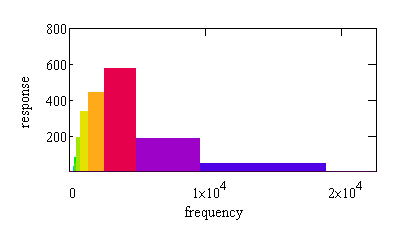
The audible range is spanned by just a few octaves, so octave analysis produces a relatively coarse categorization. Resolution is improved by breaking the octave bands into sub-octave bands, preserving the logarithmic band spacing. For the conventional case that octaves are separated into 3 parts, each successive 1/3 octave band increases in width by a factor of 1.25992. Though the relative widths are fixed mathematically, standards [3] define nominal locations for these bands — useful for labeling purposes.
The natural and efficient way to analyze the spectrum of discretely-sampled signals, an FFT, partitions the frequency spectrum linearly. An octave analysis partitions the spectrum logarithmically. Because of this fundamental clash, octave analysis is typically done by filtering methods, not FFT methods. This has its own set of problems, and every filter (whether analog or digital) must be carefully and individually designed.
An FFT-based analysis
The approach described here uses a high resolution FFT frequency analysis, and takes advantage of a peculiar mathematical quirk to align the FFT analysis and octave analysis. Completing the octave analysis is then a simple bookkeeping matter — making sure that every frequency sample in the FFT is categorized into the correct octave.
Briefly, this is the mathematical oddity: Suppose you start at normalized frequency position 1.0, and divide this into equal steps of length 1/12. This spans the frequency interval from 1.0 to 2.0 — one octave. Then, you cluster the 12 steps into a group of 3 steps, then 4 steps, then 5 steps. What you really want, however, is to span the octave interval with steps that are equal in log base 2. Calculating the logarithms, you will find that they are as follows:
  (steps)            1.0000    1.2500    1.5833    2.0000
  (log 2 steps)      0.0000    0.3218    0.6629    1.0000
  (desired)          0.0000    0.3333    0.6667    1.0000
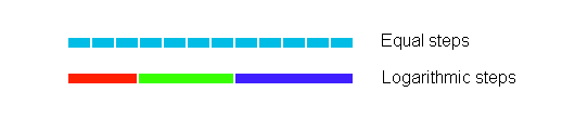
As it happens, this specially-selected set of integer-space steps in the FFT has the remarkable property of almost perfectly aligning to logarithmically equal intervals in frequency. There is just a small error in the third decimal place. It is hard to get filters calibrated this accurately... and an FFT requires no calibration.
But to take advantage of this numerical oddity, these intervals of step 3+4+5 must be correctly aligned to the FFT. In particular, the lowest octave must correspond to 12 consecutive FFT locations. If you can establish this alignment, then a set of 12 FFT locations spans the first octave, a set of 24 locations spans the second octave, a set of 48 locations spans the third octave, and so forth until you run out of spectrum terms.
The details of this alignment have been worked out. All you need to do is pick the appropriate tabulated values, provided in a detailed technical note [4]. The FFT configurations given there will guarantee that your sampled data correctly represents the desired spectrum bands, and that your analysis correctly aligns to a specific set of 1/3 octave bands that standards have defined.
Processing
Counting up the number of terms the FFT analysis needs:
12 + 24 + 48 + 96 + ...
Each term in the sum doubles the previous one. Expand this pattern out until it has 10 terms — what you need to cover the full audio spectrum — and the FFT starts to get very large. A capable FFT method is needed to analyze data blocks this size. The DAPL 3000 system includes the MIXRFFT command, which is a modeless, floating point FFT analysis capable of processing the very long data blocks needed for a successful 1/3 octave analysis.
Once the power spectrum analysis is done, there is still the problem of properly accounting for which spectrum terms fall into which octave bands. This is covered by a separate processing command, THIRDOCT. This command is not part of the DAPL 3000 system, but it is available as a separate free download [5] on this site.
Applications
You don't need any special data acquisition "toolkits" or mathematical analysis packages for this. You can read the results using the software system of your choice: a C program, DAPstudio, Excel spreadsheet, or an automated test system. The process is the same for all of them. Send your configuration scripts and receive back completed 1/3 octave results with no additional data processing required.
An example configuration is provided in the DAPstudio configuration file included with the download package [5]. This configuration runs on an xDAP 7400 data acquisition system [1] and can analyze and display up to 8 simultaneously-sampled channels covering the complete audio spectrum from 8 Hz to 22 kHz, at continuous real-time rates.
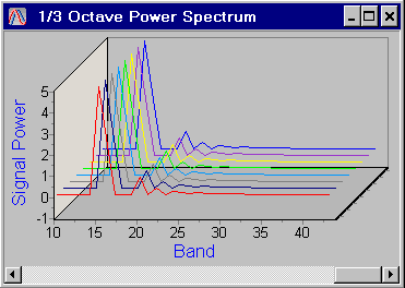
Active plot displayed by DAPstudio
Conclusion
There are other ways to perform octave analysis. If you have the time and resources, you can take advantage of some very sophisticated data acquisition and analysis packages that support 1/3 octave analysis... and much more. They do a superb job. This comes at a price, however. It is sometimes awkward to support a heavyweight data acquisition environment, and it can be nearly impossible to grind through all of the raw data while also supporting the graphical display functions in real-time. For these situations, a DAP-based system provides an economical, low-overhead alternative, with the DAP providing an extra layer of processing resources.
Footnotes and References:
- Find out more about the xDAP 7400 used for the 1/3 octave acquisition and processing.
- "Octave Analysis Explored," Kurt Veggeberg, Evaluation Engineering, August 2008, pp 40-43.
- ANSI s1.11-1986, "Specification for octave-band and fractional-octave-band analog and digital filters"
ANSI s1.11-2004, "Specification for octave-band and fractional-octave-band analog and digital filters"
IEC 1260:1995-07, "Electroacoustics - Octave Band and Fractional Octave Band Filters"
IEC 1260:1995-07 Annex A- Download a copy of the Technical Note 257 that discusses 1/3 octave applications in greater detail.
- Download a copy of the THIRDOCT processing command.
Return to the DSP page.