Time Shift Correction Filters

Home

Products

Applications

Introduction

(View more DSP information or download the preliminary implementation.)

It is common to have a number of analog signals, sampled at moderate rates, where time relationships between channels are important. For example, in beamforming applications with a microphone array, time shifts are related to the location of the audio source, which is the critical information. You don't want those time shifts confused with artificial time delays caused by discrete time sampling. A direct way to address this problem is to use simultaneous sampling hardware. This works well, avoiding the time and phase anomalies. However, simultaneous sampling hardware comes at a price, because electronic components must be dedicated to each signal line. Sometimes economics dictate a search for a less expensive alternative.

Data acquisition devices that can multiplex their conversion electronics provide a much more economical approach to data sampling, but these devices must operate serially. There is an incremental time-shift as each data channel is sampled, but this shift is very precise and predictable. Within certain limitations, a straightforward application of established digital processing techniques can provide an accurate and economical way to correct for the time and phase shifts introduced into the data by the sampling process.

Time-Shift Corrections Using the `MTSFILT` Processing Command

A processing command to apply time-shift filtering to the practical problem of aligning data samples skewed in time by multiplexed sampling is available. The MTSFILT processing command is a Multiple channel Time-Shift Filtering command that acts upon multiple data channels to produce sample streams in which the time delays inherent in multiplexed sampling are eliminated. The command has the following form.

  MTSFILT( inpipe, nchan, xover, outpipe )

where the parameters are

inpipe: a pipe containing multiplexed word data samples
nchan: the number of multiplexed channels in the data stream
xover: the oversampling present in the data set to reduce the time-shift between channels
outpipe: a pipe where the multiplexed, reconstructed word data samples are placed

Each input signal from inpipe must be at least 2x oversampled; that is, the effective sampling rate for each channel (sampling rate / the number of multiplexed channels) should be at least 4 times the highest frequency present in the signal at the input sample rate. This restriction results from the properties of the lowpass filtering used to build the interpolation filters. The data sampling rate can be increased beyond what is strictly necessary to operate the time-shift filtering, to reduce the time separation between physical samples, thus reducing the magnitude of the corrections needed, and reducing sensitivity to certain practical concerns such as disturbances and noise. The xover parameter is a positive "oversampling factor" specifying the amount of additional oversampling present in the signal. The output pipe <outpipe> receives the multiplexed results of the time-shift filtering at the desired rate after disposing of the extra samples.

Example: Suppose that a value is needed from each of 4 channels in 25 milliseconds. That is 40 microseconds to cover the four channels, or a sampling interval of 10 microseconds between data channels. A Data Acquisition Processor has plenty of capacity to sample faster than that. So the value of xover can be set to 4, and the sampling interval set to 2.5 microseconds.

Test

A configuration with five data channels requires simultaneous samples at 400 microsecond intervals, with the full theoretical Nyquist band preserved at this sample rate. Apply 4x oversampling; at this rate, the sampled data stream well below the theoretical band limits, and sampling is 100 microseconds on each channel. Because there are five channels, the multiplexing sample interval must be set to 20 microseconds. After capturing the multiplexed data, the data stream is sent to the MTSFILT command for time-shift correction. The reconstructed simultaneous-time data stream, with samples at 400 microsecond intervals on each channel, is transferred to the PC for logging.

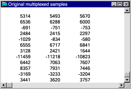
The MTSFILT command was tested with a randomized signal appropriately filtered to enforce the bandlimit restrictions. The same signal is sampled on all channels, so if the sampling were simultaneous, the values captured in each channel should be the same. When multiplexed sampling is used, it is easy to see the progression of signal changes from one channel to the next.

After processing by the MTSFILT processing command, the sample values should be all the same. Due to the limitations of the filter design, there can be small variations, but these are at the level of bit chatter in the low order bit of the analog to digital converter hardware.

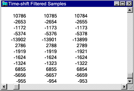
You can verify this test in the downloadable configuration for DAP Measurement Studio. After time-shift correction, the values of all samples are indistinguishable from independent simultaneous measurements.

How Does Time-Shift Filtering Work?

Transversal or "shift register" filters are completely natural for time shifting. A finite impulse response (FIR) filter is a practical implementation of this idea with a finite length array for the filter coefficients. Consider for example a degenerate FIR filter characterized by the following set of coefficients:

   ( 0.0  0.0  1.0  0.0  0.0 )

When this set of coefficients is convolved with a data stream to evaluate the filter, the center coefficient is aligned at the point of interest in the data stream, terms of the data stream and filter characteristic are multiplied pairwise, and the resulting products are summed to produce the filtered output. Clearly, the only term that has any effect is the one aligned to the 1.0 coefficient, so the new data stream is unchanged by the filtering operation.

Consider now what happens if the 1.0 value is swapped with the 0.0 value on its left side. Now the only term that aligns with a nonzero coefficient is one position older. The filter result is almost the same, except that the filter output sequence matches the original stream one sample displaced into the past. In a similar fashion, swapping the 1.0 value with the 0.0 value on its right side shifts the data stream so that output terms appear one position sooner. Shifting the filter coefficients has the effect of time-shifting the output data stream.

This works perfectly, provided that the desired time shift matches an exact integer number of sample positions. What if it does not?

Non-Integer Shifts: Signal Reconstruction and Interpolation Filters

Let's quickly review some basic theory. Shannon, Nyquist, and other pioneers of digital signal processing considered the problem of determining when a set of discrete samples of a signal is sufficient to completely characterize the original analog signal. The first fundamental and in some ways astonishing result is:

An analog signal can be perfectly and completely reconstructed, anywhere, from its discrete-time samples provided that the original signal is suitably band-limited.

That restriction is subtle. Usually the bandlimit condition cannot be guaranteed. But even so, where the violations are small, deviations from theory are small and the results are very good, as good as the original samples.

The problem of signal reconstruction is closely related to the "interpolation problem" of classical numerical analysis — to determine the approximate value of a function at any point given the function values at a discrete set of locations. For this reason, the filters for reconstructing an analog signal are also called interpolation filters.

A second extremely important theoretical result is the explicit specification of a digital filter form to perform the reconstruction perfectly. Omitting the details [1], we can simply point out:

the theoretically ideal reconstruction filter to rebuild the original signal value at any point in time is a transversal shift register filter.

It would in fact be a FIR filter except for the annoying difficulty that it is infinite. A filter with an infinite number of terms is not the sort of thing you want to evaluate in real time. Most of the terms are very small, and that suggests truncating the infinite theoretical filter to a finite length as an approximation. This must be done with care, as dropping an infinite number of terms can have unexpected side effects.

The reconstruction problem becomes much easier if we insist that the original signal is bandlimited well below theoretical Nyquist limit. Suppose that the frequency band for the original system is restricted as shown in figure 1, and then a lowpass filter as shown in figure 2 is applied. What is the result?

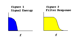
The filter has no effect, because the frequency bands that it attenuates are already completely empty. As long as this property is satisfied, other design details are arbitrary, so pick a symmetric FIR filter with a small number of filter coefficients and a flat, accurate passband.

Now pick a desired time location for reconstructing the signal. Construct the ideal interpolation filter according to theory, and apply this to the discrete signal — after the change-nothing lowpass filtering is applied. Now, the two filter operations, lowpass and interpolation, can be combined mathematically. The combination yields a filter form that has the interpolation performance of the theoretical reconstruction filter when operating upon the restricted-band signals, and can be truncated to a finite length with very little loss of accuracy.

Knowing the conditions under which efficient FIR filters can perform the signal reconstruction at any desired point in time, we are not forced to start from the general theory for designing interpolation filters. Any method that produces a good approximation to the theoretical ideal will also work well. The accompanying worksheet [2] shows a simple design method based on least squares best approximation, and this can generate practical interpolation filter designs for any desired sample location.

From Interpolation to Time Shift

Time shifting is simply a matter of selecting the position in a time sequence where the interpolation filtering is applied. By selecting an appropriately staggered time-shift for each data channel, the values of the reconstructed samples can be made to align in time, correcting the artificial time delays caused by sampling.

To summarize briefly, the values produced by the interpolation filter can be indistinguishable from values obtained by physical simultaneous sampling at those instants. However, suitable applications must :

make sure that the signal is clean and properly band limited,
oversample so that the rate is not too close to the theoretical Nyquist limit,
allow for processing delays as filtering is performed,
not expect accurate reconstructions near signal discontinuities.

The World's Most Terrifying DSP Operation

It is a well known fact that common digital filtering operations such as Butterworth IIR filtering [3] can replace the original signal samples with new sample values at the same locations [4] such that the signal is improved [5] but in all other respects there is minimal disturbance. [6] Anybody who just finished the previous sentence without flinching should check the footnotes right now to find out how it is wrong [3], wrong[4], wrong[5], and (not surprisingly) wrong[6].

In contrast to Butterworth-like filters, which distort data in a manner that is seldom well understood, the interpolation filters have a sound theoretical basis, are extremely predictable, and perform efficiently.

So please explain. Why is Butterworth-like digital filtering, despite all of its known deficiencies, applied almost without a second thought; while time-shift filtering (without those deficiencies) remains too terrifying to consider?

We certainly are baffled. But time shifting remains perhaps the most under-utilized DSP technique.

Conclusions

The MTSFILT command makes time-shift corrections easy to apply. It can't replace true simultaneous sampling, but sometimes there is good economy possible from using the digital time-shift filters with lower-cost multiplexed sampling devices. If the limitations are respected and the command is used properly, the results are indistinguishable from measurements captured by actual simultaneous sampling. In some cases, with data corrupted by low levels of random noise, despite the fact that this violates the prerequisite conditions, measurements are actually improved due to the noise reduction inherent in the filtering.

There should be no terror in applying well-suited and well-established DSP technology properly. Be very afraid about too casually applying other limited technologies presumed to be "safe" for no particularly good reason.

MTSFILT uses established DSP technology, not anything new and experimental. The only thing new is an improved package that makes it very easy to use. This demonstrates that "applying DSP" does require staying mired in mathematical theory.

If you were looking for the benefits of simultaneous sampling without the price tag, consider the MTSFILT command for your project.

Footnotes and References:

For the full details, you can try Digital Signal Processing, Alan V. Oppenheim and Ronald W. Schafer, Prentice Hall Inc., 1975, section 1.7. Any other good textbook on digital signal processing will cover this fundamental material.

A copy of a Mathcad 12 worksheet for time-shift filter designs using least squared methods is provided with the command download. (Mathcad is a registered trade name of Mathsoft Engineering and Education, Inc.) An example application of the worksheet is shown in the HTML snapshot, and you can grab all of the formulas there.

While Butterworth filters are certainly IIR filters, they are continuous-time filters and will always remain so. Some discrete time filters, notably the "max-flat designs" share some of the same properties. It is possible to map analog designs into discrete time IIR designs, but there are limits to what can be achieved this way.

The same locations? Well, not really. The shifts produced by Butterworth filters are far more drastic than you might think, and because these are a nonlinear function of frequency, you must pay the price of waveform distortions.

Filtering can never add information to a signal. Sometimes Butterworth filters "improve" the signal in the sense that the results "look smoother" and have attenuation where you need it. But it's not all improvement, if you take the distortions into account.

Don't be fooled. The only thing that a Butterworth-like filter minimizes is passband flatness in the neighborhood of zero frequency. The rest is a compromise.

Return to the DSP page. Or download the preliminary implementation.