PIDZ - PID With Zero-Shaping Control

PID Control Command

(View more Control information or download the preliminary implementation.)

This note describes a new DAP processing command for a variation of PID control. While the primary intent is to exercise and evaluate certain new features, the preliminary implementation available with this note might be useful in its current form.

If this command has features that you like, but it is missing something important, talk to us! Perhaps that feature is fundamental, and we really should have included it anyway. Perhaps it is already in the plan for the next iteration. Or perhaps you have special needs — processing speed, multiple channels, tuning, monitoring — features that we could develop for you as a custom product.

This is a work under development, not a finished product, so you must take this into account. However, we won't forbid using the command for production applications if you are willing to test vigorously and accept the risks.

PID controls in the DAPL system

The DAPL system hasn't paid much attention to PID, for good reason. Suppose you need to run 100 independent PID loops. What are you going to do with the other 90% of the DAP's processing capacity? By today's standards, PID loops require rather sparse data streams and rather little processing resource. A Data Acquisition Processor's primary purpose, most of the time, is intensive data capture and intensive processing. For everyday simple PID applications, DAP solutions tend to be overkill.

On the other hand, there are those few stubborn control loops that don't want to be simple PID applications. They are perhaps 5% of the applications and 99% of the grief. DAPs can push data through remarkably fast when lightly loaded, and they also offer outstanding configurability. Modifying a self-contained PID control module would be out of the question, but customized PID algorithms and configurations are commonplace in a DAPL solution.

One possible customization addresses control loops for which the plant tends to oscillate easily. Ordinary PID feedback control introduces a closed loop zero that aggravates any tendency to oscillate or overshoot. The system might not be able to tolerate the poorly damped transients that result every time the setpoint level is changed. Gains must be backed down to compensate, and consequently loop performance suffers. The PIDZ command provides an additional tuning option that might help control these relatively uncooperative systems.

Conventional Modifications to PID Control

For this discussion, we will start by considering a classic PID controller in the form of the ISA reference model.

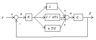
Two common modifications are made to the derivative feedback path of this conventional configuration:

For systems that are not intended to track a rapidly changing reference setpoint command level, the derivative feedback is made insensitive to transient conditions on the command input by applying it only to the output feedback. This has been a feature of the DAPL system PID commands since the earliest times.
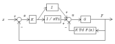
Pure derivative feedback has infinite gain at high frequencies. It is common practice to limit derivative gains using a low order lowpass "smoothing" filter. For discrete PID controllers, a pure derivative is never available in any case -- it is always an estimate, and the smoothed response helps to compensate for sampling and estimation anomalies. The DAPL system applies a smoothing filter with rolloff at about 1/10 of the Nyquist frequency. This has been a feature of DAPL PID support since year 2001.

With these modifications, the closed loop control looks like the following.

Zero Placement Control

As long as we are making changes to the PID configuration, let us consider making changes to the proportional gain paths too. As an intermediate step, let us split the effects of the proportional gain into separate paths for command and feedback. In addition, an artificial unity gain block is added to the command path. Reviewing the net flow into the summing junction leading to the plant drive signal, we can see that this configuration is completely equivalent.

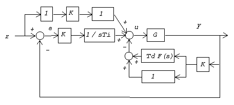
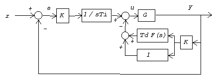
Now allow the first gain block in the proportional command path to be adjustable. Call the new gain b. If we adjust this new gain, we will get different closed loop response, but how useful is it?

To examine this, compute the transfer functions for command input response, also output disturbance rejection response.

                 K ( s b + 1/Ti ) G
Y/U  =   -----------------------------------------
            s   +   K ( s + 1/Ti + s Td F(s)) G

                          1
Y/D  =   -----------------------------------------
            s   +   K ( s + 1/Ti + s Td F(s)) G

Some observations:

The new zero shaping gain b appears only in the command response transfer function. Thus it neither helps nor harms disturbance rejection.
Disturbance rejection might receive indirect benefit. Sometimes the feedback gain can be increased after damping is improved in command input response.
The numerator factor containing the b term is the response zero introduced by PID feedback.
Making the b term smaller shifts the location of the transfer function zero to a higher frequency, where the plant response is attenuated, hence less impact on loop performance.

Let's take this to the extreme. What if we send the value of the b multiplier all the way to zero? In that case, the extra closed loop zero disappears completely, and we obtain a special configuration known as a pseudoderivative controller.

The command response transfer function is:

                     K/Ti  G
Y/U  =   -----------------------------------------
            s   +   K ( s + 1/Ti + s Td F(s)) G

It has the advantages:

No new closed loop zero is introduced.
Little or no overshoot in step response.
Doesn't require integrator anti-windup compensation.
Easy to modify for higher-order tracking accuracy.
As easy as classical PID to implement.

This is a useful alternative to classic PID. If you need faster step response and do not experience excessive overshoot, the classic PID configuration is probably better because of its faster initial rise time. If you need to control overshoot and obtain a smoother response to command inputs, the pseudoderivative configuration is probably better. You don't need to make an all-or-nothing choice, the gain parameter b is continuously adjustable.

Just as a footnote, the "pseudoderivative controller" was named (perhaps for tenuous reasons) by its inventor Richard Phelan, who described it and several variations in "Automatic Control Systems", Cornell University Press, 1977. Copies are very hard to find. The idea did not get much attention. Phelan was a mechanical engineer in an era when control theory was becoming the uncontested domain of the electrical engineers, so the academic community largely ignored it. PID advocates and suppliers had their own vested interests. Phelan tended to describe his controller with superlatives that were summarily discounted by a control community that didn't believe in ultimate solutions. A command path prefilter idea achieving roughly the same end became canonical.

Simulating PIDZ Action

Download the PIDZ module and test files. The included DAPL configuration file can be run under DAPview for Windows. It is a self contained implementation of a simulated, uncooperative plant under PID control, using the PIDZ command as the controller. Most of the listing is for generating and timing the simulation. The actual PID control part is a single line: the PIDZ command. The gain settings for the PIDZ command appear near the top of the listing. Users of DAPview for Windows can load the included workspace file to view live plots of system and controller outputs.

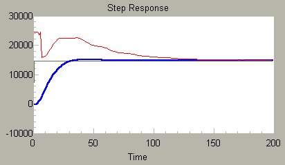
The simulation applies a step response. The goal of the PID tuning is to find feedback setting that yield a fast, smooth closed loop response to the setpoint input, while maintaining a high loop gain to keep disturbance rejection as high as possible. To run the simulation, you must select values for the PID gain parameters and then tell your software to start the configuration. Each run generates three curves: the setpoint input level, the controller drive level, and the plant output level.

This particular plant is sluggish in reaching its new setpoint level, as you can see in the following step response simulation without closed loop control.

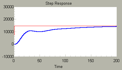
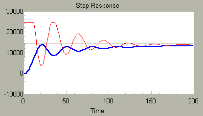
Yet, despite being so sluggish, you can see that it has a tendency to wobble. Feedback tends to excite that poorly damped mode. The response can become unstable rather easily. The following shows the response in a classic PID configuration under proportional control, with just a little integral gain for reset action.

VARIABLE  KGAIN FLOAT = 4.0
VARIABLE  TI FLOAT    =  1.0
VARIABLE  TD FLOAT    =  0.0001
VARIABLE  BGAIN FLOAT = 1.0

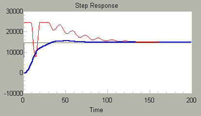
The initial gain settings can be improved quite a lot, in particular, derivative feedback to counter those oscillations, and integral feedback to bring the level to the desired setpoint more efficiently. With some experimentation, we can find a response such as the following.

VARIABLE  KGAIN FLOAT = 7
VARIABLE  TI FLOAT    = 0.05
VARIABLE  TD FLOAT    = 0.04
VARIABLE  BGAIN FLOAT = 1.0

This isn't bad, but that internal mode is bouncing the control against the upper limit and producing an erratic approach to the setpoint. Just as an experiment, let's make a complete shift, and throw the loop into pure pseudoderivative mode by setting the zero shaping parameter b to 0.0, leaving all the other tunings unchanged. It is clear that we have not drastically altered the response characteristic, but we get a slightly smoother rise time. The erratic control output is somewhat troubling, but does not seem to disturb the system output very much.

VARIABLE  KGAIN FLOAT = 7.0
VARIABLE  TI FLOAT    = 0.05
VARIABLE  TD FLOAT    = 0.04
VARIABLE  BGAIN FLOAT = 0.0

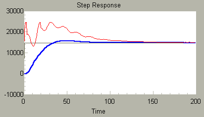
Encouraged by this smooth response, we can now try final adjustments: try to boost the gain a little for better disturbance rejection, adjust the integral term to adjust the rather minor overshoot, adjust the derivative term to control the wobble, and adjust the zero shaping parameter to give the smoothest response. When we do that, something remarkable happens.

VARIABLE  KGAIN FLOAT = 7.7
VARIABLE  TI FLOAT    = 0.041
VARIABLE  TD FLOAT    = 0.020
VARIABLE  BGAIN FLOAT = 0.29

With these settings, there is a clean step response, and also a quite smooth response from the controller as well. Where did that wobble go?

There is an approximate pole-zero cancellation, at least enough to tame most observed effects of the oscillatory mode. Don't be fooled, that mode is still there, and the system is closer to its stability margin than might appear. Nevertheless, the system performance seems quite good. This is great for somebody trying to optimize loop performance, maybe not so great for professors needing observability to prove some stability theorems.

This rather unexpected result illustrates how adjusting a transfer function zero with PIDZ can sometimes make a surprising difference in the way a feedback loop behaves.

About the PIDZ command

The attached command reference page describes the PIDZ processing command. Unlike its predecessors, this command specifies gain parameters in the manner of the ISA reference model. Applications specifying feedback gains in terms of independent P, I and D parameters in the manner of the DAPL system PID1 command need to convert to the equivalent K, Ti and Td representation as explained in the DAPL 2000 Manual. The sampling time must be specified so that the tuning parameters can be related to the sample rate. Of course, the zero-shaping b parameter is new.

The PIDZ command uses floating point for its internal calculations, to maintain consistent scaling over a wide range of sampling intervals and process rates. This version probably runs too slowly on DAP models that do not have processor hardware support for floating point.

PIDZ provides anti-windup limiting of the error integral, but does not provide supervisory control and "bumpless" gain adjustments as provided in the DAPL system's PID1 command.

To use PIDZ , you need to download the PIDZM.DLM module file, and register it with the DAPcell control panel application as a loadable system module. The PIDZ processing command will then be available every time your system is booted up.

Don't have a DAP in your test toolkit? That's a problem. If the need is urgent, call our Sales department and see if they can arrange for a demo unit for testing.