DAPL Commands as State Observers — A Hydraulic Control Application
Introduction

(View more Control information or download the preliminary implementation.)
One of the things that DAPL tasks can do well is filter data. Filters take streams of data in, and send streams of data out. They can remove information, shift information in time, or present information in different combinations.
A state filter is a kind of filter that operates on a signal containing a mix of information, yielding a separated stream for each signal component that generated the mix. Sample values in the output streams represent the current estimates of state variables. It is not possible to generate these estimates instantaneously, but it is possible to do so over time if the sources have identifiable properties that distinguish them, and if the system has suitable observability properties. Unlike frequency selective filtering, observer filters can work even if there is considerable overlap in the frequency bands of the component sources.
For purposes of control systems, it is best to take accurate and independent measurements of as many relevant variables as possible. Unfortunately, it is sometimes very difficult or very expensive to accurately measure every relevant variable. State observers can be used to "fill in" missing information to good approximation.
About Hydraulic Actuators
In this note, we consider an observer for a linear travel hydraulic actuator, as might be used in suspension or vibration testing. The following diagram summarizes the elements of the actuator system. This might look complicated, but it really isn't as bad as it seems. (The real thing is actually much worse!)
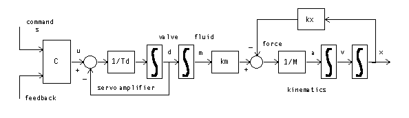
The diagram shows five "stages" that act in sequence.
- Motion commands s drive a controller, possibly incorporating feedback information.
- The controller sends control signal u to drive a high-bandwidth servo amplifier, with an internal integrator and lag time constant.
- The servo adjusts the fluid control valve to position d. This establishes the hydraulic fluid transfer rate. Hydraulic fluid mass m accumulates in the actuator cylinder.
- The fluid transfer increases pressure. Displacement of the piston within the cylinder relieves the pressure. Coefficients describe the relative effect of fluid injection and piston displacement.
- The pressure accelerates the piston and the physical mass M attached to it. Integrating acceleration a yields velocity v. Integrating velocity v yields piston position x.
This model includes many simplifications, perhaps over-simplifications. Just to point out a couple:
- other forces also act on the attached mass besides the accelerating pressure,
- the relationship between pressure and displacement is a nonlinear inverse one, not the simple addition and subtraction shown.
Still, this very simple model captures a lot of the behaviors of a real actuator system.
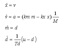
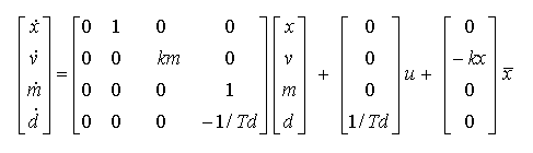
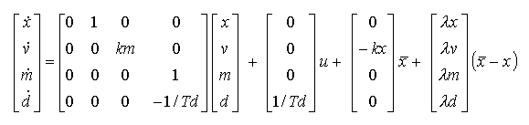
We can organize the information above in the form of differential equations.
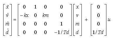
We can then organize the differential equations into the state-space form if we wish, using a matrix notation:
Motivations For the State Observer
Anything known about the actuator state could be helpful for controlling it. But not all of the information is readily accessible.
- Displacement
xis relatively fast and easy to measure with good accuracy. - Direct measurement of velocity
vis possible, but usually not very accurate. - It is almost impossible to measure the amount of fluid
min the actuator cylinder. It is possible to tap through the pressure chamber walls to measure pressure, but good accuracy is difficult. - The servo valve position
dis typically hidden and unmeasurable.
As an experiment, let's simulate a feedback system using the displacement state variable, which is easily observed. Using a modest proportional feedback gain of −0.5, we get the following step response over a 1-second time interval.
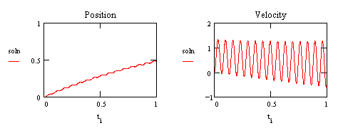
This is rather scary. We are getting the expected slow exponential approach to the desired setpoint, but look at that growing oscillation in the velocity variable — the system is unstable. Any amount of proportional gain will cause the loop to go unstable in this manner. A real system will have energy losses not represented in this model, but that tiny margin is the only thing preventing a destructive vibration.
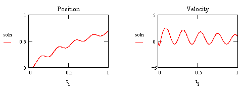
Let's contrast this with the performance that might be possible if additional states were measurable. Apply a controller that uses direct measurement of all states.
This has proportional correction −0.08, velocity feedback 0.68, fluid transfer feedback −0.0058 and servo feedback of −0.0016. It is interesting to note that the velocity feedback seems to be positive rather than negative, but after the phase shifts that result when the corrections propagate around the feedback loop, the net effect is stabilizing. The ringing is still there, but now it is damped.
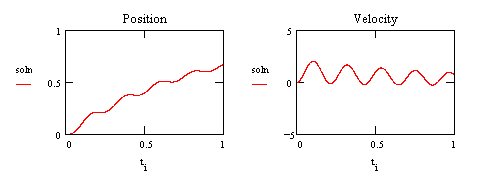
We would like to get similar results, but without the costs and complexities of measuring the extra states. Suppose we use the observer to do this, using the same gain settings for proportional, velocity, and fluid transfer feedback. We see the following.
The behavior is very much the same except for a slightly larger magnitude in the oscillation. This occurs during the start-up transient, as the observer cancels its initial state estimate errors. If the initial estimates are very good, there is less additional excitation for the oscillation, and the behavior is very much like full state feedback.
State Observers Are the Rule, Not the Exception!
You might be reluctant to consider an obscure or academic technology that is rarely used in practice. You might or might not be surprised by our claim that
MOST feedback control applications use state observers.
What evidence can we offer to support this? Very simple: Most feedback control applications use PID.
Think about it. How many systems out there have an auxiliary "derivative plug" delivering the exact derivative of the main output signal? Not many. Yet PID controllers must base their control output on that derivative. That missing derivative signal is supplied by estimating it from observed changes in the original signal.
You might argue: "Well yes, but that's estimating the derivative of the output, which is not the same thing as estimating a state variable." That is partly true, but in a state representation, the system output is functionally dependent on the system state. So estimating the output is really the same thing as estimating a system state, or more precisely, one particular combination of states. If you have lived with the peculiarities of derivative feedback over the years, you already know a lot about the nature of state observers.
Obtaining Practical Observer Equations
The scheme used by PID control does not extend well beyond the first derivative estimate. We want to consider how additional information can be used to obtain more and better state estimates.
One important way to predict state variables is to apply a mathematical model. For the case of the hydraulic actuator, we have already described such a model. In concept, if we drive this model with exactly the same command signal that drives the actual system, we should be able to predict the states the actual system will reach. Unfortunately, consider the following simulation, showing what happens if there are tiny errors in the initial state estimates, drive signal, and model coefficients.
As you can see, the model predictions and the actual states diverge rather quickly. Some kind of corrective action is needed. We can compare the outputs generated by the real system to the outputs predicted by the model, and use this difference to correct the estimates continuously over time. Using this strategy — observer model equals system model plus incremental corrections — we will now set up equations for a hydraulic actuator observer.
First, note that we have accurate measurements of the
piston position state x, so measured values of
x can be treated as external information
independent of the observer model. We retain an estimated
x term in the model, however, as this gives us
a means to detect divergence of the observer from actual
state. With this change, the observer equations become
Now we apply the correction terms.
Estimated and measured x variables
now occur in multiple locations. Combine terms, folding the
new "observer gain" terms into the earlier matrix and
vector locations.
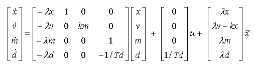
The final step is to select values of the observer gain λ coefficients so that observer prediction errors converge to zero at the desired rate. There are good and poor observer tunings, just as there are good and poor feedback loop tunings. A good tuning will adjust slowly, fast enough to keep the state estimates on track, but slow enough for low sensitivity to noise.
Example: Design for a hydraulic actuator, sampling at 10000 Hz, with half power bandwidth 500 Hz. Estimating the time constant for the 500 Hz band edge frequency
   1/(2 π 500)  --> 3.184x10⁴ sec
        --> roughly 3 time steps
look for a settling response to be much slower than this, around 300 time steps, or about 1/30 second. The disturbance should be mostly settled in about 1/10 second. We can simulate the observer model for 1/10 of a second and verify that state errors approximately converge within this time frame.
For an actuator model with the following parameters:
kx 1.8 105 lbf/in
km 2.4 105 lbf/oz
M 20 lbm
Td 3.0 10-4 sec
Sample time 1/10000
we selected the observer gains
λkx 150
λkm 14000
λM 35
λTd 1000
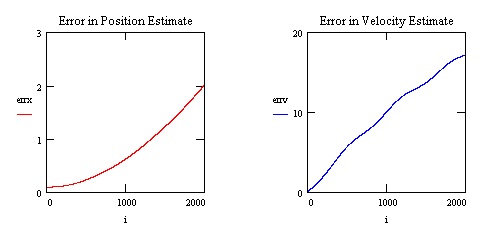
The following is a simulation of the observer error in the estimates of the position and velocity states. It can be seen that the error decays quickly and is negligible after about 1000 samples (1/10 second).
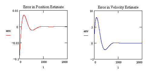
The slow response time for observer correction should not be confused with response to actuator command inputs! Only the small persistent offsets are corrected slowly. The 10000 Hz sampling rate is chosen to assure that the observer can track all state changes, without difficulty, to the 500 Hz band limit of the actuator.
We have described the observer design process in some detail because your system might need a very different model. While designing and verifying your observer, you should discover that the observer gains are non-critical, and no further tuning adjustments are needed.
Downloads
If you would like to experiment with the hydraulic
observer, it is implemented as a DAPL processing command
HYDRAULOBS. The command module can be downloaded. Pass the state
matrix, the observer gains, and the initial state to
HYDRAULOBS to initialize it. At run time, it
reads the current command and system output streams, and
generates a set of multiplexed state estimate streams. You
can run this command in parallel with an actual system
first, to gain confidence that the computations produce good
state estimates, before trying to use the command within a
feedback control loop.
Conclusions
This note has described a state observer for a particular kind of system, but the general approach covered here will work with any kind of system where a suitable model and a suitable means of incrementally correcting the model's state exist. That means, the model can be as complex as necessary.
There is not much point in using a state observer and multiple feedback control scheme if simpler observer schemes such as PID work sufficiently. However, for some systems that are somewhat hard to control, such as high-performance hydraulic actuators, PID has certain stability limitations. State observers might be helpful in overcoming those limitations. Packaged as a DAPL processing command, state observer filters are no harder to use than ordinary data filters in a DAPL processing configuration. Performance of a feedback loop using the observer often compares very well to performance using complete state measurement, but at a much lower cost for sensors and supporting instrumentation.
Footnotes and References:
- For a general survey, try Observers, Bernard Friedland, Chapter 37 in The Control Handbook, IEEE Press, 1995, William S. Levine ed. This is a rather academic treatment, but it is hard to find anything better. Let us know if you find something.
- The fact that the feedback performance was good using only three of the four observed states suggests that the observer might be more complex than necessary. You might want to investigate Reduced Order Observers: A New Algorithm and Proof, Paul Van Doren, Systems & Control Letters, 1984, pp. 243-251.
Return to the Control page. Or download the experimental implementation.