Nonlinear Adaptive Control of a Biological Reactor
Beyond PID

(View more Control information or download the preliminary implementation.)
When you have a system for which simple control strategies are not quite good enough, how can you implement something better? Data Acquisition Processor boards provide one possibility, and they can do much more than just the real-time control of the process.
Biological processes sound very easy, but as it turns out, these present just about every kind of control system nightmare other than discontinuity. The process discussed in this note is a "fed batch reactor," a process in which microorganisms are cultivated in a tank [1]. Lacking anything original, let's hypothesize that the organisms are genetically modified bacteria for manufacturing a kind of agricultural growth hormone. Liquid nutrients are added to feed the bacteria growth. The hormone is secreted into the tank as a biological waste product. To recover the product, a stream of liquid is drawn off for processing, replaced with sterile liquid. Supplemental systems regulate temperature, liquid levels, and stirring rates for the tank contents.
Figure 1: Fed batch bio-reactor process
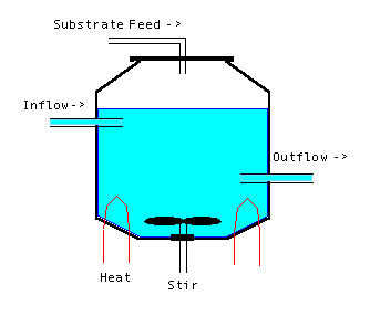
The population can sustain production when nutrients support enough new growth to balance the portion of the population drawn off with processed liquid. The most important measured variable is the population density. The primary control on the population is the substrate feed rate. This system seems like a good candidate for PID control, and in fact, PID controls have been used for such processes — but they don't work very well. The population tends to grow exponentially if fed too much, or to collapse exponentially if not fed enough.
PID control is faced with three challenges:
The further away from the balance point, the harder a PID controller pushes to establish the setpoint level. That linear kind of behavior is not well suited to the biological reactor because of its inherent volatility.
PID control works best when the signal it generates directly drives the observed system variable it is controlling. For this particular system, that direct connection is missing. Nutrient inflow accumulates, resulting in a higher growth rate; a higher growth rate then accumulates to produce a higher population density. Thus, there is a kind of double integration: the system has relative degree two. PID controls have trouble with multiple integrator systems of this sort. Actually, all controllers do.
The functional relationship between the growth rate and the nutrient density is nonlinear and not precisely known. Growth rates can vary with the stirring disturbances, variations in temperature, nutrient mix, and inexplicable dining preferences of the particular family line of organisms.
Measurable State Variables
It is presumed that there are three measurable state variables
governing the dynamics: the population density
x, the substrate (nutrient) density
s, and detritus accumulation m.
The measurements are filtered appropriately to yield accurate
state estimates. The primary control u on the
population is the "substrate feed" providing new nutrients.
Controlling With PID
Suppose that there is no model to describe internal processes
of the real system. We can still apply a heuristic control such
as PID, because we can measure the current population density
x, compare it to the desired population density
x0, and compute a correction on that basis
alone. Without any model to indicate values that the other state
variables should reach, it is difficult to derive any advantage
from them.
We cannot use PID alone to reach setpoint effectively because the gains must be kept low for stability. To establish the necessary feed levels, first apply a nutrient density and feed level that (it is believed) will support a growing population. Then allow conditions to stabilize. Let's try this first without PID control.
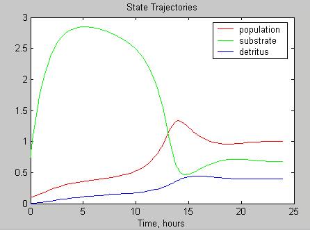
Figure 2: Constant input feedforward control
The fixed inflow strategy overfeeds the small initial population. The nutrients build up until they reach a level where they are detrimental to organism growth. Eventually, equilibrium is reached. It can be hard to guess the right feed level to get the population density desired, and it can take a very long time to settle to the right level. Otherwise, this works.
It would be much better for automatic controls to find the desired setpoint quickly and then regulate that level. We can use a PI control strategy, being careful to use very small gains. First we try adding proportional feedback gain. This is the result with gain 0.35 .
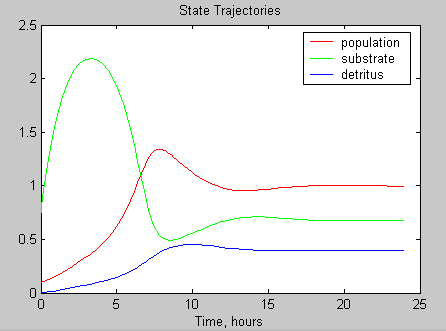
Figure 3: Feedforward control plus proportional feedback
The final convergence speed is better, but this matters little, because the initial overfeeding transient is much worse.
Integral control does not fare any better. It tends to sustain the population better, but it has the same kind of initial overfeeding problem and its settling time is degraded.
Nonlinear Bio-Reactor Controller
A better control strategy will incorporate knowledge about the system. The internal details of this design are beyond the scope of what we can describe here, but we can quickly survey some of the main features:
- nonlinear gains establish near optimal growth rate
- adaptive adjustment matches observed growth rate
- predetermined feedforward feed level not needed
- nonlinear feedback avoids transient overfeeding
- "tracking gain" for fast initial response
- "compensation gain" for cancelling nonlinear effects
- "proportional gain" for final settling control
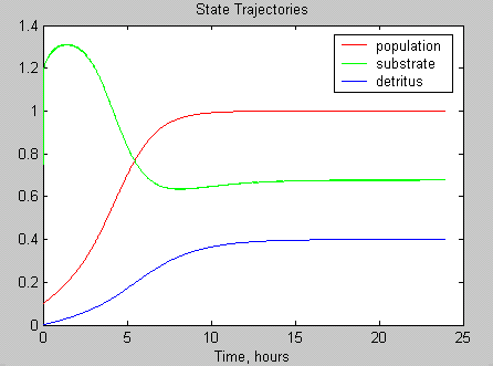
Running the nonlinear controller under the same conditions as the PID controller, here is the response.
Figure 4: Nonlinear control
Now suppose the estimated growth factor is off by about 20% at the start. We activate the adaption gain.
Figure 5: Nonlinear control with growth rate adaption
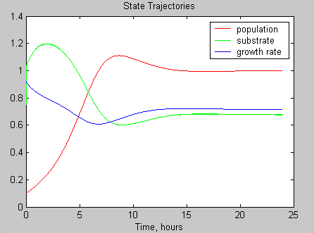
Notice that the blue trace here is the estimate of the growth rate parameter, and the mortality state is not shown. During the gross transient, the adaption law dragged the rate estimate down too low. But as the system began to stabilize, the value of the growth rate parameter stabilized too. Instead of settling in 9 hours, it took 12 hours, but the system remained in control, and also "learned" the correct growth rate factor. After settling, the adaption gain can be set to zero, and response to subsequent disturbances will be more like Figure 4.
A Mathematical Reference Model
How is it possible for the nonlinear controller to outperform the PID controller, even under imperfect information about the most critical parameter? Basically, the improved performance results from incorporating more knowledge about the internal workings of the process. In this case, the process is described by a small differential equation system. The nonlinearities and gains of the model are taken into account, "built into" the controller design. This implies a controller that is better suited to one kind of application, but limited to that one kind of application.
The population density tends to grow at a rate proportional
to the current density, and also to die off at a rate proportional
to the current density. The population is not viable unless the
growth rate exceeds the basic mortality rate. The two rates are
combined into one net growth rate, G(s), dependent
on the nutrient density s. Curve G(s)
is in general nonlinear and not well known, and we will revisit
it in a moment.
As individuals in the population die off, this results in an accumulation of detritus in the liquid, and that in turn inhibits population growth. Combining the effects of growth and inhibition yields the population density dynamic equation.
x' = G(s) x - Kx m
Nutrient density s is controlled by adjusting the
control valve u regulating inflow of substrate
materials. The population consumes the substrate nutrients. The
gain term Ks represents the proportionality between
nutrient density change and population growth.
s' = - Ks G(s) x + u
Detritus from dead organisms interferes with the healthy metabolism of the live ones, and if the accumulation is too much it can force a shutdown of the batch process. The mortality dynamic equation represents the accumulation of detritus in proportion to population density.
m' = Km x
So far, the equations describe the population dynamics in a tank with fixed content. However, some fraction of the material is drawn out in each unit of time for harvesting the hormone product. Due to the stirring of the tank contents, the drawn mixture contains parts of population, nutrient, and detritus in proportion to their densities. We include this extra draw-down rate into each of the dynamic equations to complete the population model.
  x' =  -D x  +  G(s) x    - Kx m
  s' =  -D s  -  Ks G(s) x   +  u
  m' =  -D m  +  Km x
This looks easy, but that +G(s) term in the
population equation is a positive feedback, which can make
stabilization tricky. If the growth rate exceeds the
draw-down rate D by too much, the growth tends to
explode. However, once the population gets too large, it consumes
the nutrients quickly, and then the population tends to crash.
If a wild decline wipes out the population, the batch must be
dumped and restarted.
Model Parameters - The Growth Rate
Growth has a nonlinear dependence on the nutrient density
s. We expect poor growth rates at low nutrient
density. But we also expect that metabolism is impaired if the
nutrient density is too high. In general the growth curve
is not accurately known, which means that the control loop
gain is not accurately known.
Despite various multiple-parameter models described in papers
or textbooks, there is often not enough time or information in
practice to isolate the relative influences of multiple
parameters. For our purposes here, we use a model of the
following form, with one adjustable scaling parameter
Kg.
Figure 6: Growth curve
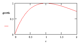
G(s) = Kg s e1-(s/smax)
The nutrient density for maximum growth is determined by
parameter smax. The value of the growth rate at
maximum is determined by the Kg parameter. These
parameters are determined from laboratory experiments. The
Kg parameter is dynamically adjusted as necessary
to scale to the actual observed growth rate.
It is presumed that the liquid draw rate D and
the nutrient feed rate u are accurately adjustable,
possibly driven by their own servo control loops.
A Quick Note About the Design
While it is what the controller does that really matters, some readers might be interested where this particular controller design came from. The controller was derived using a backstepping method[2,3,4] with matched direct parameter adaption. The design method constructs a sequence of control terms for the differential equation model and evaluates their effect, using candidate Lyapunov functions until one is found that simultaneously assures convergence of all adaption, settling, and tracking errors to zero. Lots of coffee helps.
Even though the design of the controller can be tedious, the implementation is rather easy. The section of code that does the real work of the control computation spans about 45 lines. A dense and cryptic coding style without source documentation could squeeze this to under 30 lines.
Downloads
Unfortunately, we do not have any real bio-reactors that you can borrow. (We have automatic bread makers, but those don't count.) The best we can do is run the controller against a simulation. With a little caution, perhaps you can do more than that. Be careful, this is not field proven software and there are no assurances that it will work for you.
Some configuration files are provided in the download
package. One set is in the .DAP format used by
programmed applications or DAPview for Windows. The other
equivalent set is in the .DMS format used by the new
DAPstudio package. These configurations simulate operation
of the biological fed-batch reactor in a number of scenarios.
Adjustable parameters appear at the top of each configuration.
To access these in DAPstudio, select the Processing
tab, and under that the Procedure sub-tab. You
can modify the parameter values directly in the DAPL listing
window. The configurations include:
Fixed feedforward command. Observe the effects of model parameters on the population density. Little changes can make a big difference.
Nonlinear bio-controller action. Observe the benefits of controller action in transient and settling behaviors. Also observe the sensitivity to controller gains — not very much!
Nonlinear bio-controller with good model but poor initial growth rate estimate. Observe changes in transient and settling time caused by the parameter adaption.
Nonlinear bio-controller with poor model, poor initial growth rate estimate, and adaptive correction. Observe that modelling errors have only minor effect.
Simulated reactor under PID control. See if you can find a good PID gain tuning. Then, when you think you have it, try making minor changes to the model parameters and see what happens.
The real thing... when you are ready.
To run these, you must install the BIOCTRL.DLM
downloadable DAPL system module. See the download page. Run the Data Acquisition control panel
application and go to the MODULE tab to install the module into
the DAPL system. The simulations are self-contained. If you
use the DAPstudio configurations, your simulation
results are plotted automatically. If you are not using
DAPstudio, you need to download a copy.
Just to make things a little interesting, the scenarios illustrated in this note are not fully optimized. You can tune each one for better performance. After identifying "optimized" gains, check the robustness of the control strategy by adjusting control gains and model parameters.
Are Data Acquisition Processors The Right Solution?
We have just seen an example where PID control doesn't work very well, but where a specialized controller does. If you have a system that isn't working very well, what are the alternatives? You can continue to cope with old problems, and suffer the operational costs. You can implement a DAP-based controller. Or you can build a custom controller from low-level components -- at a cost in time and effort that really makes the cost of a DAP system seem like pocket change!
For a bio-reactor system, updates are on a scale of minutes, with sampling on the order of seconds. You don't need the full computational capacity of a DAP at these speeds. But you will need:
a software environment that makes development and support of the custom control features relatively fast and easy.
additional regulation for supplementary variables. Liquid level, temperature, and stir rate will need their own regulators. Doing all of these things, simultaneously and well, can be a very tricky matter using lower level components. The extra processing capacity of the DAP can be applied to advantage — the DAPL system can handle multiple control tasks as easily as one.
long-term monitoring for long-term operation. Data will need to be collected for analyzing process performance. DAP systems can do this with no disruption to control loops, either on-demand or logged.
remote monitoring and control. These are "standard features" of the DAPcell networking support.
reliability. Rating operating systems on a scale from "A" (never crashes), to "Z" (crashes more than it runs), by the time you get to operating systems in the range of "W" you should be wary. Desktop operating systems generally tend to kill processes perceived as compromising system availability. The mouse drivers will be safe. If you have a production run that spans days or weeks, can you risk losing control? DAP systems keep your process under control even as your operating system crashes and reboots.
Footnotes and References:
- Review of Fed-Batch Fermentations: Mathematical Modelling, Parameters, and Control, Gisela Ferreira, University of Maryland Baltimore County (UMBC). You might find a copy posted online. It seems that no two authors formulate the problem exactly the same way. Perhaps this is partly because no two reactions are exactly the same?
- An Engineering Introduction to Nonlinear Control, Graham C. Goodwin (with Jose De Dona, Osvaldo J. Rojas and Michael Perrier), University of Newcastle, Australia. You may download a PDF copy from Dr. Goodwin's site, or you might find a copy in the ICCTA-2001 proceedings under the title A Brief Overview of Nonlinear Control. Recommended, a well presented survey with a painless introduction to nonlinear backstepping.
- The Control Handbook, William S. Levine, ed., 1996. In particular, check the chapter Adaptive Nonlinear Control, Miroslav Kristic´ and Petar Kokotovic´, p. 980, for a dense but rather thorough overview of the backstepping method.
- Nonlinear and Adaptive Control Design, Miroslav Kristic´, Petar Kokotovic´, Ioannis Kanellakopoulis, 1995, John Wiley and Sons. Intimidating, but if you want authority, this delivers. Includes a two-state bio-reactor control example. Excellent bibliography.
Return to the Control page. Or download the preliminary implementation.